

Bessel function
Background Information
SOS Children, an education charity, organised this selection. Click here for more information on SOS Children.
In mathematics, Bessel functions, first defined by the mathematician Daniel Bernoulli and generalized by Friedrich Bessel, are canonical solutions y(x) of Bessel's differential equation:
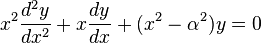
for an arbitrary real or complex number α. The most common and important special case is where α is an integer n, then α is referred to as the order of the Bessel function.
Although α and −α produce the same differential equation, it is conventional to define different Bessel functions for these two orders (e.g., so that the Bessel functions are mostly smooth functions of α). Bessel functions are also known as Cylinder functions or Cylindrical harmonics because they are found in the solution to Laplace's equation in cylindrical coordinates.
Applications
Bessel's equation arises when finding separable solutions to Laplace's equation and the Helmholtz equation in cylindrical or spherical coordinates. Bessel functions are therefore especially important for many problems of wave propagation, static potentials, and so on. In solving problems in cylindrical coordinate systems, one obtains Bessel functions of integer order (α = n); in spherical problems, one obtains half-integer orders (α = n+½). For example:
- electromagnetic waves in a cylindrical waveguide
- heat conduction in a cylindrical object.
- modes of vibration of a thin circular (or annular) artificial membrane.
- diffusion problems on a lattice.
Bessel functions also have useful properties for other problems, such as signal processing (e.g., see FM synthesis, Kaiser window, or Bessel filter).
Definitions
Since this is a second-order differential equation, there must be two linearly independent solutions. Depending upon the circumstances, however, various formulations of these solutions are convenient, and the different variations are described below.
Bessel functions of the first kind : 
Bessel functions of the first kind, denoted as Jα(x), are solutions of Bessel's differential equation that are finite at the origin (x = 0) for non-negative integer α, and diverge as x approaches zero for negative non-integer α. The solution type (e.g. integer or non-integer) and normalization of Jα(x) are defined by its properties below. For integer order solutions, it is possible to define the function by its Taylor series expansion around x = 0:
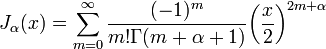
where  is the gamma function, a generalization of the factorial function to non-integer values. For non-integer α, a more general power series expansion is required. The graphs of Bessel functions look roughly like oscillating sine or cosine functions that decay proportionally to 1/√x (see also their asymptotic forms below), although their roots are not generally periodic, except asymptotically for large x. (The Taylor series indicates that
  is the derivative of
  , much like
  is the derivative of
  ; more generally, the derivative of
  can be expressed in terms of
  by the identities below.)

For non-integer α, the functions  and
and  are linearly independent, and are therefore the two solutions of the differential equation. On the other hand, for integer order
  , the following relationship is valid:
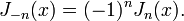
This means that the two solutions are no longer linearly independent. In this case, the second linearly independent solution is then found to be the Bessel function of the second kind, as discussed below.
Bessel's integrals
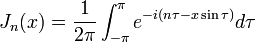
Another definition of the Bessel function, for integer values of  , is possible using an integral representation:
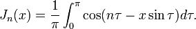
This was the approach that Bessel used, and from this definition he derived several properties of the function.
Another integral representation is:
Relation to hypergeometric series
The Bessel functions can be expressed in terms of the hypergeometric series as
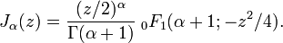
This expression is related to the development of Bessel functions in terms of the Bessel-Clifford function.
Bessel functions of the second kind : 
The Bessel functions of the second kind, denoted by Yα(x), are solutions of the Bessel differential equation. They are singular ( infinite) at the origin (x = 0).

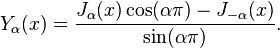
Yα(x) is sometimes also called the Neumann function, and is occasionally denoted instead by Nα(x). For non-integer α, it is related to Jα(x) by:
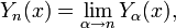
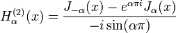
In the case of integer order n, the function is defined by taking the limit as a non-integer α tends to n':
which has the result (in integral form)
![Y_n(x) =
\frac{1}{\pi} \int_{0}^{\pi} \sin(x \sin\theta - n\theta)d\theta
- \frac{1}{\pi} \int_{0}^{\infty}
\left[ e^{n t} + (-1)^n e^{-n t} \right]
e^{-x \sinh t} dt.](../../images/208/20863.png)
For the case of non-integer α, the definition of Yα(x) is redundant (as is clear from its definition above). On the other hand, when α is an integer, Yα(x) is the second linearly independent solution of Bessel's equation; moreover, as was similarly the case for the functions of the first kind, the following relationship is valid:
Both Jα(x) and Yα(x) are holomorphic functions of x on the complex plane cut along the negative real axis. When α is an integer, there is no branch point, and the Bessel functions are entire functions of x. If x is held fixed, then the Bessel functions are entire functions of α.
Hankel functions : 
Another important formulation of the two linearly independent solutions to Bessel's equation are the Hankel functions Hα(1)(x) and Hα(2)(x), defined by:
where i is the imaginary unit. These linear combinations are also known as Bessel functions of the third kind; they are two linearly independent solutions of Bessel's differential equation. The Hankel functions of the first and second kind are used to express outward- and inward-propagating cylindrical wave solutions of the cylindrical wave equation, respectively (or vice versa, depending on the sign convention for the frequency). They are named after Hermann Hankel.
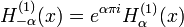
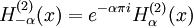
Using the previous relationships they can be expressed as:
if α is an integer, the limit has to be calculated. The following relationships are valid, whether α is an integer or not:
Modified Bessel functions : 
The Bessel functions are valid even for complex arguments x, and an important special case is that of a purely imaginary argument. In this case, the solutions to the Bessel equation are called the modified Bessel functions (or occasionally the hyperbolic Bessel functions) of the first and second kind, and are defined by:
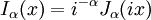
These are chosen to be real-valued for real arguments x. The series expansion for Iα(x) is thus similar to that for Jα(x), but without the alternating (-1)m factor.
Iα(x) and Kα(x) are the two linearly independent solutions to the modified Bessel's equation:

Unlike the ordinary Bessel functions, which are oscillating as functions of a real argument, Iα and Kα are exponentially growing and decaying functions, respectively. Like the ordinary Bessel function Jα, the function Iα goes to zero at x=0 for α > 0 and is finite at x=0 for α=0. Analogously, Kα diverges at x=0.
 |
 |
The modified Bessel function of the second kind has also been called by the now-rare names:
- Basset function
- modified Bessel function of the third kind
- MacDonald function
Spherical Bessel functions : 


When solving the Helmholtz equation in spherical coordinates by separation of variables, the radial equation has the form:
![x^2 \frac{d^2 y}{dx^2} + 2x \frac{dy}{dx} + [x^2 - n(n+1)]y = 0.](../../images/209/20907.png)
The two linearly independent solutions to this equation are called the spherical Bessel functions jn and yn, and are related to the ordinary Bessel functions Jn and Yn by:

 is also denoted
  or ηn; some authors call these functions the spherical Neumann functions.
The spherical Bessel functions can also be written as:
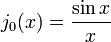
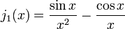
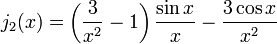
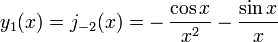
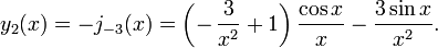
The first spherical Bessel function  is also known as the (unnormalized) sinc function. The first few spherical Bessel functions are:
and
There are also spherical analogues of the Hankel functions:
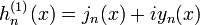
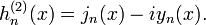
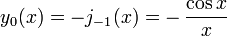
In fact, there are simple closed-form expressions for the Bessel functions of half-integer order in terms of the standard trigonometric functions, and therefore for the spherical Bessel functions. In particular, for non-negative integers n:
and hn(2) is the complex-conjugate of this (for real x). It follows, for example, that j0(x) = sin(x)/x and y0(x) = -cos(x)/x, and so on.
Riccati-Bessel functions : 
Riccati-Bessel functions only slightly differ from spherical Bessel functions:


They satisfy the differential equation:
![x^2 \frac{d^2 y}{dx^2} + [x^2 - n (n+1)] y = 0](../../images/209/20927.png)
This differential equation, and the Riccati-Bessel solutions, arises in the problem of scattering of electromagnetic waves by a sphere, known as Mie scattering after the first published solution by Mie (1908). See e.g. Du (2004) for recent developments and references.
Following Debye (1909), the notation  is sometimes used instead of
  .
.
Asymptotic forms
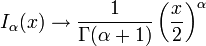
The Bessel functions have the following asymptotic forms for non-negative α. For small arguments  , one obtains:
![Y_\alpha(x) \rightarrow \left\{ \begin{matrix}
\frac{2}{\pi} \left[ \ln (x/2) + \gamma \right] & \mbox{if } \alpha=0 \\ \\
-\frac{\Gamma(\alpha)}{\pi} \left( \frac{2}{x} \right) ^\alpha & \mbox{if } \alpha > 0
\end{matrix} \right.](../../images/209/20932.png)
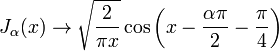
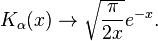
where γ is the Euler-Mascheroni constant (0.5772...) and Γ denotes the gamma function. For large arguments 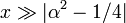 , they become:
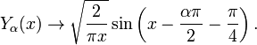
(For α=1/2 these formulas are exact; see the spherical Bessel functions above.) Asymptotic forms for the other types of Bessel function follow straightforwardly from the above relations. For example, for large , the modified Bessel functions become:
while for small arguments , they become:

Properties
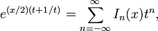
For integer order α = n, Jn is often defined via a Laurent series for a generating function:
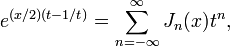
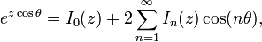
an approach used by P. A. Hansen in 1843. (This can be generalized to non-integer order by contour integration or other methods.) Another important relation for integer orders is the Jacobi-Anger identity:
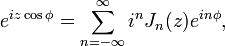
which is used to expand a plane wave as a sum of cylindrical waves, or to find the Fourier series of a tone modulated FM signal.
The functions Jα, Yα, Hα(1), and Hα(2) all satisfy the recurrence relations:
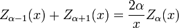
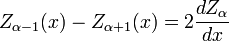
where Z denotes J, Y, H(1), or H(2). (These two identities are often combined, e.g. added or subtracted, to yield various other relations.) In this way, for example, one can compute Bessel functions of higher orders (or higher derivatives) given the values at lower orders (or lower derivatives). In particular, it follows that:
![\left( \frac{d}{x dx} \right)^m \left[ x^\alpha Z_{\alpha} (x) \right] = x^{\alpha - m} Z_{\alpha - m} (x)](../../images/209/20944.png)
![\left( \frac{d}{x dx} \right)^m \left[ \frac{Z_\alpha (x)}{x^\alpha} \right] = (-1)^m \frac{Z_{\alpha + m} (x)}{x^{\alpha + m}}](../../images/209/20945.png)
Modified Bessel functions follow similar relations :
and
The recurrence relation reads
where Cα denotes Iα or eαπiKα. These recurrence relations are useful for discrete diffusion problems.
Because Bessel's equation becomes Hermitian (self-adjoint) if it is divided by x, the solutions must satisfy an orthogonality relationship for appropriate boundary conditions. In particular, it follows that:
![\int_0^1 x J_\alpha(x u_{\alpha,m}) J_\alpha(x u_{\alpha,n}) dx
= \frac{\delta_{m,n}}{2} [J_{\alpha+1}(u_{\alpha,m})]^2
= \frac{\delta_{m,n}}{2} [J_{\alpha}'(u_{\alpha,m})]^2,](../../images/209/20950.png)
where α > -1, δm,n is the Kronecker delta, and uα,m is the m-th zero of Jα(x). This orthogonality relation can then be used to extract the coefficients in the Fourier-Bessel series, where a function is expanded in the basis of the functions Jα(x uα,m) for fixed α and varying m. (An analogous relationship for the spherical Bessel functions follows immediately.)
Another orthogonality relation is the closure equation:
for α > -1/2 and where δ is the Dirac delta function. This property is used to construct an arbitrary function from a series of Bessel functions by means of the Hankel transform. For the spherical Bessel functions the orthogonality relation is:
for α > 0.
Another important property of Bessel's equations, which follows from Abel's identity, involves the Wronskian of the solutions:
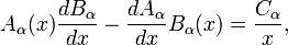
where Aα and Bα are any two solutions of Bessel's equation, and Cα is a constant independent of x (which depends on α and on the particular Bessel functions considered). For example, if Aα = Jα and Bα = Yα, then Cα is 2/π. This also holds for the modified Bessel functions; for example, if Aα = Iα and Bα = Kα, then Cα is -1.
(There are a large number of other known integrals and identities that are not reproduced here, but which can be found in the references.)
Multiplication theorem
The Bessel functions obey a multiplication theorem
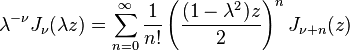
where  and
and  may be taken as arbitrary complex numbers. A similar form may be given for
  and etc. See