Correlation and dependence

Related subjects: Mathematics

Did you know...

Arranging a Wikipedia selection for schools in the developing world without internet was an initiative by SOS Children. Sponsor a child to make a real difference.

This article is about the correlation coefficient between two variables. The term correlation can also mean the cross-correlation of two functions or electron correlation in molecular systems.

Several sets of (x, y) points, with the correlation coefficient of x and y for each set. Note that the correlation reflects the noisiness and direction of a linear relationship (top row), but not the slope of that relationship (middle), nor many aspects of nonlinear relationships (bottom). N.B.: the figure in the centre has a slope of 0 but in that case the correlation coefficient is undefined because the variance of Y is zero.

In probability theory and statistics, correlation, (often measured as a correlation coefficient) , indicates the strength and direction of a linear relationship between two random variables. In general statistical usage, correlation or co-relation refers to the departure of two variables from independence. In this broad sense there are several coefficients, measuring the degree of correlation, adapted to the nature of data.

A number of different coefficients are used for different situations. The best known is the Pearson product-moment correlation coefficient, which is obtained by dividing the covariance of the two variables by the product of their standard deviations. Despite its name, it was first introduced by Francis Galton.

Pearson's product-moment coefficient

Mathematical properties

The correlation coefficient ρ_{X, Y} between two random variables X and Y with expected values μ_X and μ_Y and standard deviations σ_X and σ_Y is defined as:

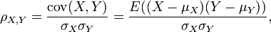
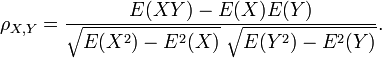
$\rho_{X,Y}={\mathrm{cov}(X,Y) \over \sigma_X \sigma_Y} ={E((X-\mu_X)(Y-\mu_Y)) \over \sigma_X\sigma_Y},$

where E is the expected value operator and cov means covariance. Since μ_X = E(X), σ_X² = E(X²) − E²(X) and likewise for Y, we may also write

$\rho_{X,Y}=\frac{E(XY)-E(X)E(Y)}{\sqrt{E(X^2)-E^2(X)}~\sqrt{E(Y^2)-E^2(Y)}}.$

The correlation is defined only if both of the standard deviations are finite and both of them are nonzero. It is a corollary of the Cauchy-Schwarz inequality that the correlation cannot exceed 1 in absolute value.

The correlation is 1 in the case of an increasing linear relationship, −1 in the case of a decreasing linear relationship, and some value in between in all other cases, indicating the degree of linear dependence between the variables. The closer the coefficient is to either −1 or 1, the stronger the correlation between the variables.

If the variables are independent then the correlation is 0, but the converse is not true because the correlation coefficient detects only linear dependencies between two variables. Here is an example: Suppose the random variable X is uniformly distributed on the interval from −1 to 1, and Y = X². Then Y is completely determined by X, so that X and Y are dependent, but their correlation is zero; they are uncorrelated. However, in the special case when X and Y are jointly normal, uncorrelatedness is equivalent to independence.

A correlation between two variables is diluted in the presence of measurement error around estimates of one or both variables, in which case disattenuation provides a more accurate coefficient.

Geometric Interpretation of correlation

The correlation coefficient can also be viewed as the cosine of the angle between the two vectors of samples drawn from the two random variables.

Caution: This method only works with centered data, i.e., data which have been shifted by the sample mean so as to have an average of zero. Some practitioners prefer an uncentered (non-Pearson-compliant) correlation coefficient. See the example below for a comparison.

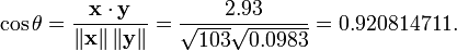
As an example, suppose five countries are found to have gross national products of 1, 2, 3, 5, and 8 billion dollars, respectively. Suppose these same five countries (in the same order) are found to have 11%, 12%, 13%, 15%, and 18% poverty. Then let x and y be ordered 5-element vectors containing the above data: x = (1, 2, 3, 5, 8) and y = (0.11, 0.12, 0.13, 0.15, 0.18).

By the usual procedure for finding the angle between two vectors (see dot product), the uncentered correlation coefficient is:

$\cos \theta = \frac { \bold{x} \cdot \bold{y} } { \left\| \bold{x} \right\| \left\| \bold{y} \right\| } = \frac { 2.93 } { \sqrt { 103 } \sqrt { 0.0983 } } = 0.920814711.$

Note that the above data were deliberately chosen to be perfectly correlated: y = 0.10 + 0.01 x. The Pearson correlation coefficient must therefore be exactly one. Centering the data (shifting x by E(x) = 3.8 and y by E(y) = 0.138) yields x = (−2.8, −1.8, −0.8, 1.2, 4.2) and y = (−0.028, −0.018, −0.008, 0.012, 0.042), from which

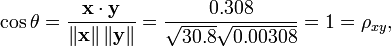
$\cos \theta = \frac { \bold{x} \cdot \bold{y} } { \left\| \bold{x} \right\| \left\| \bold{y} \right\| } = \frac { 0.308 } { \sqrt { 30.8 } \sqrt { 0.00308 } } = 1 = \rho_{xy},$

as expected.

Motivation for the form of the coefficient of correlation

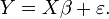
Another motivation for correlation comes from inspecting the method of simple linear regression. As above, X is the vector of independent variables, $x_i$ , and Y of the dependent variables, $y_i$ , and a simple linear relationship between X and Y is sought, through a least-squares method on the estimate of Y:

$\ Y = X\beta + \varepsilon.\,$

Then, the equation of the least-squares line can be derived to be of the form:

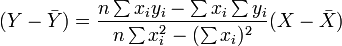
$(Y - \bar{Y}) = \frac{n\sum x_iy_i-\sum x_i\sum y_i} {n\sum x_i^2-(\sum x_i)^2} (X - \bar{X})$

which can be rearranged in the form:

$(Y - \bar{Y})=\frac{r s_y}{s_x} (X-\bar{X})$

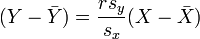
where r has the familiar form mentioned above :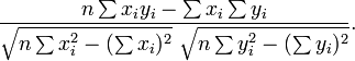 $\frac{n\sum x_iy_i-\sum x_i\sum y_i} {\sqrt{n\sum x_i^2-(\sum x_i)^2}~\sqrt{n\sum y_i^2-(\sum y_i)^2}}.$

Interpretation of the size of a correlation

Correlation	Negative	Positive
Small	−0.3 to −0.1	0.1 to 0.3
Medium	−0.5 to −0.3	0.3 to 0.5
Large	−1.0 to −0.5	0.5 to 1.0

Several authors have offered guidelines for the interpretation of a correlation coefficient. Cohen (1988), for example, has suggested the following interpretations for correlations in psychological research, in the table on the right.

As Cohen himself has observed, however, all such criteria are in some ways arbitrary and should not be observed too strictly. This is because the interpretation of a correlation coefficient depends on the context and purposes. A correlation of 0.9 may be very low if one is verifying a physical law using high-quality instruments, but may be regarded as very high in the social sciences where there may be a greater contribution from complicating factors.

Along this vein, it is important to remember that "large" and "small" should not be taken as synonyms for "good" and "bad" in terms of determining that a correlation is of a certain size. For example, a correlation of 1.0 or −1.0 indicates that the two variables analyzed are equivalent modulo scaling. Scientifically, this more frequently indicates a trivial result than an earth-shattering one. For example, consider discovering a correlation of 1.0 between how many feet tall a group of people are and the number of inches from the bottom of their feet to the top of their heads.

Non-parametric correlation coefficients

Pearson's correlation coefficient is a parametric statistic and when distributions are not normal it may be less useful than non-parametric correlation methods, such as Chi-square, Point biserial correlation, Spearman's ρ and Kendall's τ. They are a little less powerful than parametric methods if the assumptions underlying the latter are met, but are less likely to give distorted results when the assumptions fail.

Other measures of dependence among random variables

To get a measure for more general dependencies in the data (also nonlinear) it is better to use the correlation ratio which is able to detect almost any functional dependency, or the entropy-based mutual information/ total correlation which is capable of detecting even more general dependencies. The latter are sometimes referred to as multi-moment correlation measures, in comparison to those that consider only 2nd moment (pairwise or quadratic) dependence.

The polychoric correlation is another correlation applied to ordinal data that aims to estimate the correlation between theorised latent variables.

Copulas and correlation

The information given by a correlation coefficient is not enough to define the dependence structure between random variables; to fully capture it we must consider a copula between them. The correlation coefficient completely defines the dependence structure only in very particular cases, for example when the cumulative distribution functions are the multivariate normal distributions. In the case of elliptic distributions it characterizes the (hyper-)ellipses of equal density, however, it does not completely characterize the dependence structure (for example, the a multivariate t-distribution's degrees of freedom determine the level of tail dependence).

Correlation matrices

The correlation matrix of n random variables X₁, ..., X_n is the n × n matrix whose i,j entry is corr(X_i, X_j). If the measures of correlation used are product-moment coefficients, the correlation matrix is the same as the covariance matrix of the standardized random variables X_i /SD(X_i) for i = 1, ..., n. Consequently it is necessarily a positive-semidefinite matrix.

The correlation matrix is symmetric because the correlation between $X_i$ and $X_j$ is the same as the correlation between $X_j$ and $X_i$ .

Removing correlation

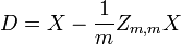
It is always possible to remove the correlation between zero-mean random variables with a linear transform, even if the relationship between the variables is nonlinear. Suppose a vector of n random variables is sampled m times. Let X be a matrix where $X_{i,j}$ is the jth variable of sample i. Let $Z_{r,c}$ be an r by c matrix with every element 1. Then D is the data transformed so every random variable has zero mean, and T is the data transformed so all variables have zero mean, unit variance, and zero correlation with all other variables. The transformed variables will be uncorrelated, even though they may not be independent.

$D = X -\frac{1}{m} Z_{m,m} X$

$T = D (D^T D)^{-\frac{1}{2}}$

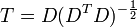
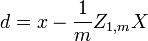
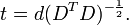
where an exponent of -1/2 represents the matrix square root of the inverse of a matrix. The covariance matrix of T will be the identity matrix. If a new data sample x is a row vector of n elements, then the same transform can be applied to x to get the transformed vectors d and t:

$d = x - \frac{1}{m} Z_{1,m} X$

$t = d (D^T D)^{-\frac{1}{2}}.$

Common misconceptions about correlation

Correlation and causality

The conventional dictum that " correlation does not imply causation" means that correlation cannot be validly used to infer a causal relationship between the variables. This dictum should not be taken to mean that correlations cannot indicate causal relations. However, the causes underlying the correlation, if any, may be indirect and unknown. Consequently, establishing a correlation between two variables is not a sufficient condition to establish a causal relationship (in either direction).

Here is a simple example: hot weather may cause both crime and ice-cream purchases. Therefore crime is correlated with ice-cream purchases. But crime does not cause ice-cream purchases and ice-cream purchases do not cause crime.

A correlation between age and height in children is fairly causally transparent, but a correlation between mood and health in people is less so. Does improved mood lead to improved health? Or does good health lead to good mood? Or does some other factor underlie both? Or is it pure coincidence? In other words, a correlation can be taken as evidence for a possible causal relationship, but cannot indicate what the causal relationship, if any, might be.

Correlation and linearity

Four sets of data with the same correlation of 0.81

While Pearson correlation indicates the strength of a linear relationship between two variables, its value alone may not be sufficient to evaluate this relationship, especially in the case where the assumption of normality is incorrect.

The image on the right shows scatterplots of Anscombe's quartet, a set of four different pairs of variables created by Francis Anscombe. The four $y$ variables have the same mean (7.5), standard deviation (4.12), correlation (0.81) and regression line ( $y = 3 + 0.5x$ ). However, as can be seen on the plots, the distribution of the variables is very different. The first one (top left) seems to be distributed normally, and corresponds to what one would expect when considering two variables correlated and following the assumption of normality. The second one (top right) is not distributed normally; while an obvious relationship between the two variables can be observed, it is not linear, and the Pearson correlation coefficient is not relevant. In the third case (bottom left), the linear relationship is perfect, except for one outlier which exerts enough influence to lower the correlation coefficient from 1 to 0.81. Finally, the fourth example (bottom right) shows another example when one outlier is enough to produce a high correlation coefficient, even though the relationship between the two variables is not linear.

These examples indicate that the correlation coefficient, as a summary statistic, cannot replace the individual examination of the data.

Computing correlation accurately in a single pass

The following algorithm (in pseudocode) will calculate Pearson correlation with good numerical stability.

sum_sq_x = 0
sum_sq_y = 0
sum_coproduct = 0
mean_x = x[1]
mean_y = y[1]
for i in 2 to N:
    sweep = (i - 1.0) / i
    delta_x = x[i] - mean_x
    delta_y = y[i] - mean_y
    sum_sq_x += delta_x * delta_x * sweep
    sum_sq_y += delta_y * delta_y * sweep
    sum_coproduct += delta_x * delta_y * sweep
    mean_x += delta_x / i
    mean_y += delta_y / i 
pop_sd_x = sqrt( sum_sq_x / N )
pop_sd_y = sqrt( sum_sq_y / N )
cov_x_y = sum_coproduct / N
correlation = cov_x_y / (pop_sd_x * pop_sd_y)

Retrieved from " http://en.wikipedia.org/w/index.php?title=Correlation_and_dependence&oldid=199055311"