Curl (mathematics)

Related subjects: Mathematics

Background to the schools Wikipedia

SOS Children made this Wikipedia selection alongside other schools resources. Sponsoring children helps children in the developing world to learn too.

In vector calculus, curl (or: rotor) is a vector operator that shows a vector field's "rate of rotation"; that is, the direction of the axis of rotation and the magnitude of the rotation. It can also be described as the circulation density.

"Rotation" and "circulation" are used here for properties of a vector function of position, regardless of their possible change in time.

A vector field which has zero curl everywhere is called irrotational.

The alternative terminology rotor and alternative notation (used in many European countries) is $\operatorname{rot}(\mathbf{F})$ are often used for curl and $\operatorname{curl}(\mathbf{F})$ .

Coordinate-invariant Definition as a Circulation Density

The component of $\operatorname{curl}(\mathbf{F})$ in the direction of unit vector $\mathbf{\hat u}$ is the limit of a line integral per unit area of $\mathbf{F}$ , namely the following integral over the closed curve $\partial S^{(2)}$ . This closed curve is in a plane normal to $\mathbf{\hat u}$ :

$\mathbf{\hat u}_{|\,(\,S^{(2)}\perp\mathbf \hat u\,)}\cdot\operatorname{curl}(\mathbf{F}) = \lim_{S^{(2)} \rightarrow 0} \frac{1}{|S^{(2)}|} \oint_{\partial S^{(2)}} \mathbf{F} \cdot d\mathbf{l}$

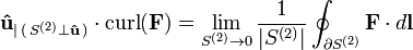
Now to calculate components of $\operatorname{curl}(\mathbf{F})$ for example in Cartesian coordinates, replace $\mathbf{\hat u}$ with unit vectors i, j and k.

This defines not only the curl in a way free of any coordinates, but makes also visible that it is a circulation density.

Stokes's theorem (see below) can directly be derived from it and the representation in special coordinates can be explicitly obtained.

Usage

In mathematics the curl is defined as:

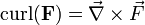
$\operatorname{curl}(\mathbf{F}) = \vec{\nabla} \times \vec{F}$

where F is the vector field to which the curl is being applied. Although the version on the right is strictly an abuse of notation, it is still useful as a mnemonic if we take $\nabla$ as a vector differential operator del or nabla. Such notation involving operators is common in physics and algebra.

Expanded in Cartesian coordinates, $\vec{\nabla} \times \vec{F}$ is, for F composed of [F_x, F_y, F_z]:

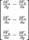
$\begin{bmatrix} {\frac{\partial F_z}{\partial y}} - {\frac{\partial F_y}{\partial z}} \\ \\ {\frac{\partial F_x}{\partial z}} - {\frac{\partial F_z}{\partial x}}\\ \\ {\frac{\partial F_y}{\partial x}} - {\frac{\partial F_x}{\partial y}} \end{bmatrix}$

Although expressed in terms of coordinates, the result is invariant under proper rotations of the coordinate axes but the result inverts under reflection.

A simple representation of the expanded form of the curl is:

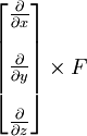
$\begin{bmatrix} {\frac{\partial}{\partial x}} \\ \\ {\frac{\partial}{\partial y}} \\ \\ {\frac{\partial}{\partial z}} \end{bmatrix} \times F$

that is, del cross F, or as the determinant of the following matrix:

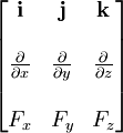
$\begin{bmatrix} \mathbf{i} & \mathbf{j} & \mathbf{k} \\ \\ {\frac{\partial}{\partial x}} & {\frac{\partial}{\partial y}} & {\frac{\partial}{\partial z}} \\ \\ F_x & F_y & F_z \end{bmatrix}$

where i, j, and k are the unit vectors for the x-, y-, and z-axes, respectively.

In Einstein notation, with the Levi-Civita symbol it is written as:

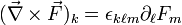
$(\vec{\nabla} \times \vec{F} )_k = \epsilon_{k\ell m} \partial_\ell F_m$

or as:

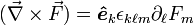
$(\vec{\nabla} \times \vec{F} ) = \boldsymbol{\hat{e}}_k\epsilon_{k\ell m} \partial_\ell F_m$

for unit vectors: $\boldsymbol{\hat{e}}_k$ , k=1,2,3 corresponding to $\boldsymbol{\hat{x}}, \boldsymbol{\hat{y}}$ , and $\boldsymbol{\hat{z}}$ respectively.

Using the exterior derivative, it is written simply as:

$dF\,$

Taking the exterior derivative of a vector field does not result in another vector field, but a 2-form or bivector field, properly written as $P\,(dx \wedge dy) + Q\,(dy \wedge dz) + R\,(dz \wedge dx)$ .

Since bivectors are generally considered less intuitive than ordinary vectors, the R³- dual : $*dF\,$ is commonly used instead (where $*\,$ denotes the Hodge star operator). This is a chiral operation, producing a pseudovector that takes on opposite values in left-handed and right-handed coordinate systems.

Interpreting the curl

The curl of vector field tells us about the rotation the field has at any point. The magnitude of the curl tells us how much rotation there is. The direction tells us, by the right-hand rule (four fingers of the right hand are curled in the direction of the motion and the thumb points in the direction of the rotation) about which axis the field is rotating.

A commonly used device for thinking about curl is the paddle wheel. If we were to place a very small paddle wheel at a point in the vector field in question and treat the drawn vectors and their lengths as currents in a river with magnitude and direction, whichever way the paddle wheel would tend to turn is the direction of the curl at that point. For example, if two currents are trying to rotate the wheel in opposite directions, the stronger one (the longer vector) will win.

Examples

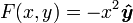
A simple vector field

Take the vector field constructed using unit vectors

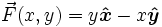$\vec{F}(x,y)=y\boldsymbol{\hat{x}}-x\boldsymbol{\hat{y}}$ .

Its plot looks like this:

Simply by visual inspection, we can see that the field is rotating. If we stick a paddle wheel anywhere, we see immediately its tendency to rotate clockwise. Using the right-hand rule, we expect the curl to be into the page. If we are to keep a right-handed coordinate system, into the page will be in the negative z direction.

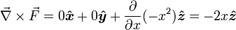
If we do the math and find the curl:

$\vec{\nabla} \times \vec{F} =0\boldsymbol{\hat{x}}+0\boldsymbol{\hat{y}}+ [{\frac{\partial}{\partial x}}(-x) -{\frac{\partial}{\partial y}} y]\boldsymbol{\hat{z}}=-2\boldsymbol{\hat{z}}$

Which is indeed in the negative z direction, as expected. In this case, the curl is actually a constant, irrespective of position. The "amount" of rotation in the above vector field is the same at any point (x,y). Plotting the curl of F isn't very interesting:

A more involved example

Suppose we now consider a slightly more complicated vector field:

$F(x,y)=-x^2\boldsymbol{\hat{y}}$ .

Its plot:

We might not see any rotation initially, but if we closely look at the right, we see a larger field at, say, x=4 than at x=3. Intuitively, if we placed a small paddle wheel there, the larger "current" on its right side would cause the paddlewheel to rotate clockwise, which corresponds to a curl in the negative z direction. By contrast, if we look at a point on the left and placed a small paddle wheel there, the larger "current" on its left side would cause the paddlewheel to rotate counterclockwise, which corresponds to a curl in the positive z direction. Let's check out our guess by doing the math:

$\vec{\nabla} \times \vec{F} =0\boldsymbol{\hat{x}}+0\boldsymbol{\hat{y}}+ {\frac{\partial}{\partial x}}(-x^2) \boldsymbol{\hat{z}}=-2x\boldsymbol{\hat{z}}$

Indeed the curl is in the positive z direction for negative x and in the negative z direction for positive x, as expected. Since this curl is not the same at every point, its plot is a bit more interesting:

Curl of F with the x=0 plane emphasized in dark blue

We note that the plot of this curl has no dependence on y or z (as it shouldn't) and is in the negative z direction for positive x and in the positive z direction for negative x.

Three common examples

Consider the example ∇ × [ v × F ]. Using Cartesian coordinates, it can be shown that

$\mathbf{ \nabla \times} \left( \mathbf{v \times F} \right) = \left[ \left( \mathbf{ \nabla \cdot F } \right) + \mathbf{F \cdot \nabla} \right] \mathbf{v}- \left[ \left( \mathbf{ \nabla \cdot v } \right) + \mathbf{v \cdot \nabla} \right] \mathbf{F} \ .$

In the case where the vector field v and ∇ are interchanged:

$\mathbf{v \ \times } \left( \mathbf{ \nabla \times F} \right) =\nabla_F \left( \mathbf{v \cdot F } \right) - \left( \mathbf{v \cdot \nabla } \right) \mathbf{ F} \ ,$

which introduces the Feynman subscript notation ∇_F, which means the subscripted gradient operates on only the factor F.

Another example is ∇ × [ ∇ × F ]. Using Cartesian coordinates, it can be shown that:

$\nabla \times \left( \mathbf{\nabla \times F} \right) = \mathbf{\nabla} (\mathbf{\nabla \cdot F}) - \nabla^2 \mathbf{F} \ ,$

which, with some head-scratching, can be construed as a special case of the first example with the substitution v → ∇.

Descriptive examples

In a tornado the winds are rotating about the eye, and a vector field showing wind velocities would have a non-zero curl at the eye, and possibly elsewhere (see vorticity).
In a vector field that describes the linear velocities of each individual part of a rotating disk, the curl will have a constant value on all parts of the disk.
If velocities of cars on a freeway were described with a vector field, and the lanes had different speed limits, the curl on the borders between lanes would be non-zero.
Faraday's law of induction, one of Maxwell's equations, can be expressed very simply using curl. It states that the curl of an electric field is equal to the opposite of the time rate of change of the magnetic field.

Retrieved from " http://en.wikipedia.org/w/index.php?title=Curl_(mathematics)&oldid=207251585"

We provide Linux to the World