

Fundamental theorem of calculus
Did you know...
SOS Children made this Wikipedia selection alongside other schools resources. Visit the SOS Children website at http://www.soschildren.org/
The fundamental theorem of calculus specifies the relationship between the two central operations of calculus, differentiation and integration.
The first part of the theorem, sometimes called the first fundamental theorem of calculus, shows that an indefinite integration can be reversed by a differentiation.
The second part, sometimes called the second fundamental theorem of calculus, allows one to compute the definite integral of a function by using any one of its infinitely many antiderivatives. This part of the theorem has invaluable practical applications, because it markedly simplifies the computation of definite integrals.
The first published statement and proof of a restricted version of the fundamental theorem was by James Gregory (1638-1675). Isaac Barrow proved the first completely general version of the theorem, while Barrow's student Isaac Newton (1643–1727) completed the development of the surrounding mathematical theory. Gottfried Leibniz (1646–1716) systematized the knowledge into a calculus for infinitesimal quantities.
Intuition
Intuitively, the theorem simply states that the sum of infinitesimal changes in a quantity over time (or some other quantity) add up to the net change in the quantity.
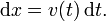
To comprehend this statement, we will start with an example. Suppose a particle travels in a straight line with its position given by x(t) where t is time and x(t) means that x is a function of t. The derivative of this function is equal to the infinitesimal change in quantity, dx, per infinitesimal change in time, dt (of course, the derivative itself is dependent on time). Let us define this change in distance per change in time as the speed v of the particle. In Leibniz's notation:

Rearranging this equation, it follows that:
By the logic above, a change in x ( ) is the sum of the infinitesimal changes dx. It is also equal to the sum of the infinitesimal products of the derivative and time. This infinite summation is integration; hence, the integration operation allows the recovery of the original function from its derivative. As one can reasonably infer, this operation works in reverse as we can differentiate the result of our integral to recover the original derivative.
Formal statements
There are two parts to the Fundamental Theorem of Calculus. Loosely put, the first part deals with the derivative of an antiderivative, while the second part deals with the relationship between antiderivatives and definite integrals.
First part
This part is sometimes referred to as First Fundamental Theorem of Calculus.
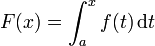
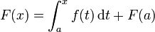
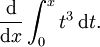
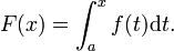
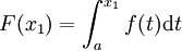
Let f be a continuous real-valued function defined on a closed interval [a, b]. Let F be the function defined, for all x in [a, b], by
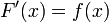
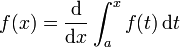
Then, F is differentiable on [a, b], and for every x in [a, b],
 .
.
The operation  is a definite integral with variable upper limit, and its result F(x) is one of the infinitely many antiderivatives of f.
Second part
This part is sometimes referred to as Second Fundamental Theorem of Calculus.
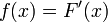
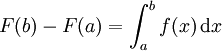
Let f be a continuous real-valued function defined on a closed interval [a, b]. Let F be an antiderivative of f, that is one of the infinitely many functions such that, for all x in [a, b],
 .
.
Then
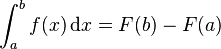 .
.
Corollary
Let f be a real-valued function defined on a closed interval [a, b]. Let F be a function such that, for all x in [a, b],
Then, for all x in [a, b],
and
 .
.
Examples
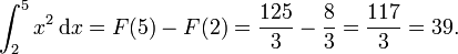
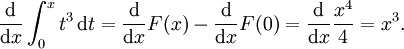
As an example, suppose you need to calculate

Here,  and we can use
  as the antiderivative. Therefore:
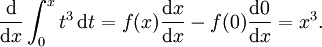
Or, more generally, suppose you need to calculate
Here,  and we can use
  as the antiderivative. Therefore:
But this result could have been found much more easily as
Proof
Suppose that
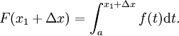
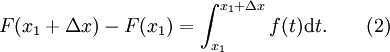
Let there be two numbers x1 and x1 + Δx in [a, b]. So we have
and
Subtracting the two equations gives

It can be shown that
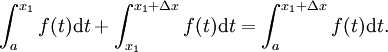
- (The sum of the areas of two adjacent regions is equal to the area of both regions combined.)
Manipulating this equation gives
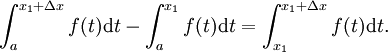
Substituting the above into (1) results in
According to the mean value theorem for integration, there exists a c in [x1, x1 + Δx] such that
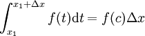 .
.
Substituting the above into (2) we get
 .
.
Dividing both sides by Δx gives
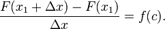
- Notice that the expression on the left side of the equation is Newton's difference quotient for F at x1.
Take the limit as Δx → 0 on both sides of the equation.
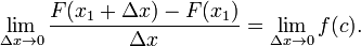
The expression on the left side of the equation is the definition of the derivative of F at x1.
To find the other limit, we will use the squeeze theorem. The number c is in the interval [x1, x1 + Δx], so x1 ≤ c ≤ x1 + Δx.
Also,  and
and  .
.
Therefore, according to the squeeze theorem,
Substituting into (3), we get
The function f is continuous at c, so the limit can be taken inside the function. Therefore, we get
 .
.
which completes the proof.
(Leithold et al, 1996)
Alternative proof
This is a limit proof by Riemann sums.
Let f be continuous on the interval [a, b], and let F be an antiderivative of f. Begin with the quantity
 .
.
Let there be numbers
- x1, ..., xn
such that
 .
.
It follows that
 .
.
Now, we add each F(xi) along with its additive inverse, so that the resulting quantity is equal:
![\begin{matrix} F(b) - F(a) & = & F(x_n)\,+\,[-F(x_{n-1})\,+\,F(x_{n-1})]\,+\,\ldots\,+\,[-F(x_1) + F(x_1)]\,-\,F(x_0) \, \\
& = & [F(x_n)\,-\,F(x_{n-1})]\,+\,[F(x_{n-1})\,+\,\ldots\,-\,F(x_1)]\,+\,[F(x_1)\,-\,F(x_0)] \, \end{matrix}](../../images/62/6206.png)
The above quantity can be written as the following sum:
![F(b) - F(a) = \sum_{i=1}^n [F(x_i) - F(x_{i-1})] \qquad (1)](../../images/62/6207.png)
Next we will employ the mean value theorem. Stated briefly,
Let F be continuous on the closed interval [a, b] and differentiable on the open interval (a, b). Then there exists some c in (a, b) such that
It follows that

The function F is differentiable on the interval [a, b]; therefore, it is also differentiable and continuous on each interval xi-1. Therefore, according to the mean value theorem (above),

Substituting the above into (1), we get
![F(b) - F(a) = \sum_{i=1}^n [F'(c_i)(x_i - x_{i-1})].](../../images/62/6211.png)
The assumption implies 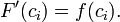 Also,
Also,  can be expressed as of partition
  .
.
![F(b) - F(a) = \sum_{i=1}^n [f(c_i)(\Delta x_i)] \qquad (2)](../../images/62/6215.png)

Notice that we are describing the area of a rectangle, with the width times the height, and we are adding the areas together. Each rectangle, by virtue of the Mean Value Theorem, describes an approximation of the curve section it is drawn over. Also notice that  does not need to be the same for any value of , or in other words that the width of the rectangles can differ. What we have to do is approximate the curve with
  rectangles. Now, as the size of the partitions get smaller and n increases, resulting in more partitions to cover the space, we will get closer and closer to the actual area of the curve.
By taking the limit of the expression as the norm of the partitions approaches zero, we arrive at the Riemann integral. That is, we take the limit as the largest of the partitions approaches zero in size, so that all other partitions are smaller and the number of partitions approaches infinity.
So, we take the limit on both sides of (2). This gives us
![\lim_{\| \Delta \| \to 0} F(b) - F(a) = \lim_{\| \Delta \| \to 0} \sum_{i=1}^n [f(c_i)(\Delta x_i)]\,.](../../images/62/6225.png)
Neither F(b) nor F(a) is dependent on ||Δ||, so the limit on the left side remains F(b) - F(a).
![F(b) - F(a) = \lim_{\| \Delta \| \to 0} \sum_{i=1}^n [f(c_i)(\Delta x_i)]](../../images/62/6226.png)
The expression on the right side of the equation defines an integral over f from a to b. Therefore, we obtain
which completes the proof.
Generalizations
We don't need to assume continuity of f on the whole interval. Part I of the theorem then says: if f is any Lebesgue integrable function on [a, b] and x0 is a number in [a, b] such that f is continuous at x0, then
is differentiable for x = x0 with F'(x0) = f(x0). We can relax the conditions on f still further and suppose that it is merely locally integrable. In that case, we can conclude that the function F is differentiable almost everywhere and F'(x) = f(x) almost everywhere. This is sometimes known as Lebesgue's differentiation theorem.
Part II of the theorem is true for any Lebesgue integrable function f which has an antiderivative F (not all integrable functions do, though).
The version of Taylor's theorem which expresses the error term as an integral can be seen as a generalization of the Fundamental Theorem.
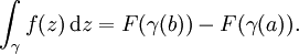
There is a version of the theorem for complex functions: suppose U is an open set in C and f: U → C is a function which has a holomorphic antiderivative F on U. Then for every curve γ: [a, b] → U, the curve integral can be computed as
The fundamental theorem can be generalized to curve and surface integrals in higher dimensions and on manifolds.
One of the most powerful statements in this direction is Stokes' theorem.