Gaussian elimination

Related subjects: Mathematics

Did you know...

Arranging a Wikipedia selection for schools in the developing world without internet was an initiative by SOS Children. See http://www.soschildren.org/sponsor-a-child to find out about child sponsorship.

In linear algebra, Gaussian elimination is an algorithm that can be used to determine the solutions of a system of linear equations, to find the rank of a matrix, and to calculate the inverse of an invertible square matrix. Gaussian elimination is named after German mathematician and scientist Carl Friedrich Gauss.

Elementary row operations are used throughout the algorithm. The algorithm has two parts, each of which considers the rows of the matrix in order. The first part reduces the matrix to row echelon form while the second reduces the matrix further to reduced row echelon form. The first part alone is sufficient for many applications.

A related but less-efficient algorithm, Gauss–Jordan elimination, brings a matrix to reduced row echelon form in one pass.

History

The method of Gaussian elimination appears in Chapter Eight, Rectangular Arrays, of the important Chinese mathematical text Jiuzhang suanshu or The Nine Chapters on the Mathematical Art. Its use is illustrated in eighteen problems, with two to five equations. The first reference to the book by this title is dated to 179 CE, but parts of it were written as early as approximately 150 BCE.

However, the method was invented in Europe independently. It is named after the mathematician Carl Friedrich Gauss.

Algorithm overview

The process of Gaussian elimination has two parts. The first part (Forward Elimination) reduces a given system to either triangular or echelon form, or results in a degenerate equation with no solution, indicating the system has no solution. This is accomplished through the use of elementary row operations. The second step uses back substitution to find the solution of the system above.

Stated equivalently for matrices, the first part reduces a matrix to row echelon form using elementary row operations while the second reduces it to reduced row echelon form, or row canonical form.

Another point of view, which turns out to be very useful to analyze the algorithm, is that Gaussian elimination computes a matrix decomposition. The three elementary row operations used in the Gaussian elimination (multiplying rows, switching rows, and adding multiples of rows to other rows) amount to multiplying the original matrix with invertible matrices from the left. The first part of the algorithm computes an LU decomposition, while the second part writes the original matrix as the product of a uniquely determined invertible matrix and a uniquely determined reduced row-echelon matrix.

Example

Suppose the goal is to find and describe the solution(s), if any, of the following system of linear equations:

$2x + y - z = 8 \quad (L_1)$

$-3x - y + 2z = -11 \quad (L_2)$

$-2x + y + 2z = -3 \quad (L_3)$

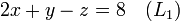
The algorithm is as follows: eliminate $x$ from all equations below $L_1$ , and then eliminate $y$ from all equations below $L_2$ . This will put the system into triangular form. Then, using back-substitution, each unknown can be solved for.

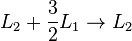
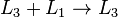
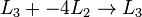
In our example, we eliminate $x$ from $L_2$ by adding $\begin{matrix}\frac{3}{2}\end{matrix} L_1$ to $L_2$ , and then we eliminate $x$ from $L_3$ by adding $L_1$ to $L_3$ . Formally:

$L_2 + \frac{3}{2}L_1 \rightarrow L_2$

$L_3 + L_1 \rightarrow L_3$

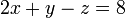
The result is:

$2x + y - z = 8 \,$

$\frac{1}{2}y + \frac{1}{2}z = 1 \,$

$2y + z = 5 \,$

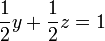
Now we eliminate $y$ from $L_3$ by adding $-4L_2$ to $L_3$ :

$L_3 + -4L_2 \rightarrow L_3$

The result is:

$2x + y - z = 8 \,$

$\frac{1}{2}y + \frac{1}{2}z = 1 \,$

$-z = 1 \,$

This result is a system of linear equations in triangular form, and so the first part of the algorithm is complete.

The second part, back-substitution, consists of solving for the unknowns in reverse order. Thus, we can easily see that

$z = -1 \quad (L_3)$

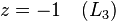
Then, $z$ can be substituted into $L_2$ , which can then be solved easily to obtain

$y = 3 \quad (L_2)$

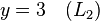
Next, $z$ and $y$ can be substituted into $L_1$ , which can be solved to obtain

$x = 2 \quad (L_1)$

Thus, the system is solved.

This algorithm works for any system of linear equations. It is possible that the system cannot be reduced to triangular form, yet still have at least one valid solution: for example, if $y$ had not occurred in $L_2$ and $L_3$ after our first step above, the algorithm would have been unable to reduce the system to triangular form. However, it would still have reduced the system to echelon form. In this case, the system does not have a unique solution, as it contains at least one free variable. The solution set can then be expressed parametrically (that is, in terms of the free variables, so that if values for the free variables are chosen, a solution will be generated).

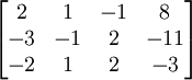
In practice, one does not usually deal with the actual systems in terms of equations but instead makes use of the augmented matrix (which is also suitable for computer manipulations). This, then, is the Gaussian Elimination algorithm applied to the augmented matrix of the system above, beginning with:

$\begin{bmatrix} 2 & 1 & -1 & 8 \\ -3 & -1 & 2 & -11 \\ -2 & 1 & 2 & -3 \end{bmatrix}$

which, at the end of the first part of the algorithm looks like this:

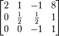
$\begin{bmatrix} 2 & 1 & -1 & 8 \\ 0 & \frac{1}{2} & \frac{1}{2} & 1 \\ 0 & 0 & -1 & 1 \end{bmatrix}$

That is, it is in row echelon form.

At the end of the algorithm, we are left with

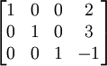
$\begin{bmatrix} 1 & 0 & 0 & 2 \\ 0 & 1 & 0 & 3 \\ 0 & 0 & 1 & -1 \end{bmatrix}$

That is, it is in reduced row echelon form, or row canonical form.

Other applications

Finding the inverse of a matrix

Suppose $A$ is a $n \times n$ matrix and you need to calculate its inverse. The $n \times n$ identity matrix is augmented to the right of $A$ , forming a $n \times 2n$ matrix (the block matrix $B = [A, I]$ ). Through application of elementary row operations and the Gaussian elimination algorithm, the left block of $B$ can be reduced to the identity matrix $I$ , which leaves $A^{-1}$ in the right block of $B$ .

If the algorithm is unable to reduce $A$ to triangular form, then $A$ is not invertible.

In practice, inverting a matrix is rarely required. Most of the time, one is really after the solution of a particular system of linear equations.

The general algorithm to compute ranks and bases

The Gaussian elimination algorithm can be applied to any $m \times n$ matrix $A$ . If we get "stuck" in a given column, we move to the next column. In this way, for example, some $6 \times 9$ matrices can be transformed to a matrix that has a reduced row echelon form like

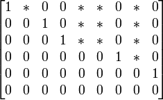
$\begin{bmatrix} 1 & * & 0 & 0 & * & * & 0 & * & 0 \\ 0 & 0 & 1 & 0 & * & * & 0 & * & 0 \\ 0 & 0 & 0 & 1 & * & * & 0 & * & 0 \\ 0 & 0 & 0 & 0 & 0 & 0 & 1 & * & 0 \\ 0 & 0 & 0 & 0 & 0 & 0 & 0 & 0 & 1 \\ 0 & 0 & 0 & 0 & 0 & 0 & 0 & 0 & 0 \end{bmatrix}$

(the *'s are arbitrary entries). This echelon matrix $T$ contains a wealth of information about $A$ : the rank of $A$ is 5 since there are 5 non-zero rows in $T$ ; the vector space spanned by the columns of $A$ has a basis consisting of the first, third, fourth, seventh and ninth column of $A$ (the columns of the ones in $T$ ), and the *'s tell you how the other columns of $A$ can be written as linear combinations of the basis columns.

Analysis

Gaussian elimination on an n × n matrix requires approximately 2n³ / 3 operations. So it has a complexity of $\mathcal{O}(n^3)\,$ .

This algorithm can be used on a computer for systems with thousands of equations and unknowns. However, the cost becomes prohibitive for systems with millions of equations. These large systems are generally solved using iterative methods. Specific methods exist for systems whose coefficients follow a regular pattern (see system of linear equations).

The Gaussian elimination can be performed over any field.

Gaussian elimination is numerically stable for diagonally dominant or positive-definite matrices. For general matrices, Gaussian elimination is usually considered to be stable in practice if you use partial pivoting as described below, even though there are examples for which it is unstable.

Pseudocode

As explained above, Gaussian elimination writes a given m × n matrix A uniquely as a product of an invertible m × m matrix S and a row-echelon matrix T. Here, S is the product of the matrices corresponding to the row operations performed.

The formal algorithm to compute $T$ from $A$ follows. We write $A[i,j]$ for the entry in row $i$ , column $j$ in matrix $A$ . The transformation is performed "in place", meaning that the original matrix $A$ is lost and successively replaced by $T$ .

i := 1
j := 1
while (i ≤ m and j ≤ n) do
  Find pivot in column j, starting in row i:
  maxi := i
  for k := i+1 to m do
    if abs(A[k,j]) > abs(A[maxi,j]) then
      maxi := k
    end if
  end for
  if A[maxi,j] ≠ 0 then
    swap rows i and maxi, but do not change the value of i
    Now A[i,j] will contain the old value of A[maxi,j].
    divide each entry in row i by A[i,j]
    Now A[i,j] will have the value 1.
    for u := i+1 to m do
      subtract A[u,j] * row i from row u
      Now A[u,j] will be 0, since A[u,j] - A[i,j] * A[u,j] = A[u,j] - 1 * A[u,j] = 0.
    end for
    i := i + 1
  end if
  j := j + 1
end while

This algorithm differs slightly from the one discussed earlier, because before eliminating a variable, it first exchanges rows to move the entry with the largest absolute value to the "pivot position". Such a pivoting procedure improves the numerical stability of the algorithm; some variants are also in use.

The column currently being transformed is called the pivot column. Proceed from left to right, letting the pivot column be the first column, then the second column, etc. and finally the last column before the vertical line. For each pivot column, do the following two steps before moving on to the next pivot column:

Locate the diagonal element in the pivot column. This element is called the pivot. The row containing the pivot is called the pivot row. Divide every element in the pivot row by the pivot to get a new pivot row with a 1 in the pivot position.
Get a 0 in each position below the pivot position by subtracting a suitable multiple of the pivot row from each of the rows below it.

Upon completion of this procedure the augmented matrix will be in row-echelon form and may be solved by back-substitution.

Retrieved from " http://en.wikipedia.org/w/index.php?title=Gaussian_elimination&oldid=199193881"

We provide Linux to the World