

Histogram
Background Information
SOS Children produced this website for schools as well as this video website about Africa. Sponsoring children helps children in the developing world to learn too.

In statistics, a histogram is a graphical display of tabulated frequencies. A histogram is the graphical version of a table that shows what proportion of cases fall into each of several or many specified categories. The histogram differs from a bar chart in that it is the area of the bar that denotes the value, not the height, a crucial distinction when the categories are not of uniform width (Lancaster, 1974). The categories are usually specified as non-overlapping intervals of some variable. The categories (bars) must be adjacent.
The word histogram is derived from Greek: histos 'anything set upright' (as the masts of a ship, the bar of a loom, or the vertical bars of a histogram); gramma 'drawing, record, writing'. The histogram is one of the seven basic tools of quality control, which also include the Pareto chart, check sheet, control chart, cause-and-effect diagram, flowchart, and scatter diagram. A generalization of the histogram is kernel smoothing techniques. This will construct a very smooth probability density function from the supplied data.
Examples
As an example we consider data collected by the U.S. Census Bureau on time to travel to work (2000 census, , Table 5). The census found that there were 124 million people who work outside of their homes. People were asked how long it takes them to get to work, and their responses were divided into categories: less than 5 minutes, more than 5 minutes and less than 10, more than 10 minutes and less than 15, and so on. The tables shows the numbers of people per category in thousands, so that 4,180 means 4,180,000.
The data in the following tables are displayed graphically by histograms. An interesting feature of both diagrams is the spike in the 30 minutes category. It seems likely that this is an artifact: half an hour is a common unit of informal time measurement, so people whose travel times were perhaps a little less than, or a little greater than 30 minutes might be inclined to answer "30 minutes". This rounding is a common phenomenon when collecting data from people.

| Interval | Width | Quantity | Quantity/width |
|---|---|---|---|
| 0 | 5 | 4180 | 836 |
| 5 | 5 | 13687 | 2737 |
| 10 | 5 | 18618 | 3723 |
| 15 | 5 | 19634 | 3926 |
| 20 | 5 | 17981 | 3596 |
| 25 | 5 | 7190 | 1438 |
| 30 | 5 | 16369 | 3273 |
| 35 | 5 | 3212 | 642 |
| 40 | 5 | 4122 | 824 |
| 45 | 15 | 9200 | 613 |
| 60 | 30 | 6461 | 215 |
| 90 | 60 | 3435 | 57 |
This histogram shows the number of cases per unit interval so that the height of each bar is equal to the proportion of total people in the survey who fall into that category. The area under the curve represents the total number of cases (124 million). This type of histogram shows absolute numbers.

| Interval | Width | Quantity (Q) | Q/total/width |
|---|---|---|---|
| 0 | 5 | 4180 | 0.0067 |
| 5 | 5 | 13687 | 0.0220 |
| 10 | 5 | 18618 | 0.0300 |
| 15 | 5 | 19634 | 0.0316 |
| 20 | 5 | 17981 | 0.0289 |
| 25 | 5 | 7190 | 0.0115 |
| 30 | 5 | 16369 | 0.0263 |
| 35 | 5 | 3212 | 0.0051 |
| 40 | 5 | 4122 | 0.0066 |
| 45 | 15 | 9200 | 0.0049 |
| 60 | 30 | 6461 | 0.0017 |
| 90 | 60 | 3435 | 0.0004 |
This histogram differs from the first only in the vertical scale. The height of each bar is the decimal percentage of the total that each category represents, and the total area of all the bars is equal to 1, the decimal equivalent of 100%. The curve displayed is a simple density estimate. This version shows proportions, and is also known as a unit area histogram.
In other words a histogram represents a frequency distribution by means of rectangles whose widths represent class intervals and whose areas are proportional to the corresponding frequencies. They only place the bars together to make it easier to compare data.
Activities and demonstrations
The SOCR resource pages contain a number of hands-on interactive activities demonstrating the concept of a Histogram, histogram construction and manipulation using Java applets and charts.
Mathematical definition
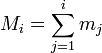
In a more general mathematical sense, a histogram is a mapping  that counts the number of observations that fall into various disjoint categories (known as bins), whereas the graph of a histogram is merely one way to represent a histogram. Thus, if we let
  be the total number of observations and
  be the total number of bins, the histogram meets the following conditions:

Cumulative histogram
A cumulative histogram is a mapping that counts the cumulative number of observations in all of the bins up to the specified bin. That is, the cumulative histogram  of a histogram is defined as:
Number of bins and width
There is no "best" number of bins, and different bin sizes can reveal different features of the data. Some theoreticians have attempted to determine an optimal number of bins, but these methods generally make strong assumptions about the shape of the distribution. You should always experiment with bin widths before choosing one (or more) that illustrate the salient features in your data.
The number of bins can be calculated directly, or from a suggested bin width  :
:
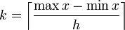
The braces indicate the ceiling function.
- Sturges' formula
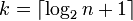
which implicitly bases the bin sizes on the range of the data, and can perform poorly if  .
.
- Scott's choice

where is the common bin width, and  is the sample standard deviation.
- Freedman-Diaconis' choice
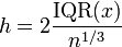
which is based on the interquartile range
Continuous data
The idea of a histogram can be generalized to continuous data. Let  (see Lebesgue space), then the cumulative histogram operator
  can be defined by:
 with only finitely many intervals of monotony this can be rewritten as
 .
.
 is undefined if
  is the value of a stationary point.