

Least squares
Background to the schools Wikipedia
SOS Children offer a complete download of this selection for schools for use on schools intranets. Sponsor a child to make a real difference.
The method of least squares, also known as regression analysis, is used to model numerical data obtained from observations by adjusting the parameters of a model so as to get an optimal fit of the data. The best fit is characterized by the sum of squared residuals have its least value, a residual being the difference between an observed value and the value given by the model. The method was first described by Carl Friedrich Gauss around 1794. Least squares corresponds to the maximum likelihood criterion if the experimental errors have a normal distribution. Regression analysis is available in most statistical software packages.

History
Context
The method of least squares grew out of the fields of astronomy and geodesy as scientists and mathematicians sought to provide solutions to the challenges of navigating the Earth's oceans during the Age of Exploration. The accurate description of the behaviour of celestial bodies was key to enabling ships to sail in open seas where before sailors had to rely on land sightings to determine the positions of their ships.
The method was the culmination of several advances that took place during the course of the eighteenth century:
- The combination of different observations taken under the same conditions as opposed to simply trying one's best to observe and record a single observation accurately. This approach was notably used by Tobias Mayer while studying the librations of the moon.
- The combination of different observations as being the best estimate of the true value; errors decrease with aggregation rather than increase, perhaps first expressed by Roger Cotes.
- The combination of different observations taken under different conditions as notably performed by Roger Joseph Boscovich in his work on the shape of the earth and Pierre-Simon Laplace in his work in explaining the differences in motion of Jupiter and Saturn.
- The development of a criterion that can be evaluated to determine when the solution with the minimum error has been achieved, developed by Laplace in his Method of Situation.
The method itself

Carl Friedrich Gauss is credited with developing the fundamentals of the basis for least-squares analysis in 1795 at the age of eighteen.
An early demonstration of the strength of Gauss's method came when it was used to predict the future location of the newly discovered asteroid Ceres. On January 1st, 1801, the Italian astronomer Giuseppe Piazzi discovered Ceres and was able to track its path for 40 days before it was lost in the glare of the sun. Based on this data, it was desired to determine the location of Ceres after it emerged from behind the sun without solving the complicated Kepler's nonlinear equations of planetary motion. The only predictions that successfully allowed Hungarian astronomer Franz Xaver von Zach to relocate Ceres were those performed by the 24-year-old Gauss using least-squares analysis.
Gauss did not publish the method until 1809, when it appeared in volume two of his work on celestial mechanics, Theoria Motus Corporum Coelestium in sectionibus conicis solem ambientium. In 1829, Gauss was able to state that the least-squares approach to regression analysis is optimal in the sense that in a linear model where the errors have a mean of zero, are uncorrelated, and have equal variances, the best linear unbiased estimators of the coefficients is the least-squares estimators. This result is known as the Gauss-Markov theorem.
The idea of least-squares analysis was also independently formulated by the Frenchman Adrien-Marie Legendre in 1805 and the American Robert Adrain in 1808.
Problem statement
The objective consists of adjusting the parameters of a model function so as to best fit a data set. A simple data set consists of m points (data pairs)  , i=1,...,m, where
  is an independent variable and
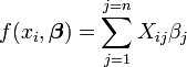
  is a dependent variable whose value is found by observation. The model function has the form
  , where the n adjustable parameters are held in the vector
  . We wish to find those parameter values for which the model "best" fits the data. The least squares method defines "best" as when the sum, S, of squared residuals

is a minimum. A residual is defined as the difference between the values of the dependent variable and the model.

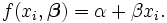
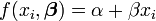
An example of a model is that of the straight line. Denoting the intercept as  and the slope as
  , the model function is given by
See linear least squares#Example for a fully worked out example of this model.
A data point may consist of more than one independent variable. For an example, when fitting a plane to a set of height measurements, the plane is a function of two independent variables, x and z, say. In the most general case there may be one or more independent variables and one or more dependent variables at each data point.
Solving the least squares problem
Least squares problems fall into two categories, linear and non-linear. The linear least squares problem has a closed form solution, but the non-linear problem has to be solved by iterative refinement; at each iteration the system is approximated by a linear one, so the core calculation is similar in both cases.
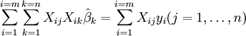
The minimum of the sum of squares is found by setting the gradient to zero. Since the model contains n parameters there are n gradient equations.
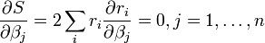
and since 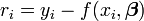 the gradient equations become
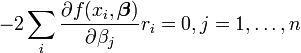
The gradient equations apply to all least squares problems. Each particular problem requires particular expressions for the model and its partial derivatives.
Linear least squares
The system is a linear one when the model comprises a linear combination of the parameters.
The coefficients  are constants or functions of the independent variable, xi.
Since 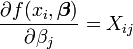 and
and 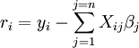 the gradient equations become
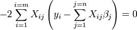
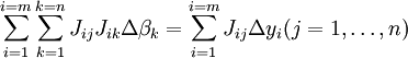
which, on rearrangement, become n simultaneous linear equations, the normal equations.
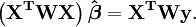
The normal equations are written in matrix notation as
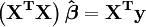
Solution of the normal equations yields the least squares estimators, , of the parameter values. See linear least squares (example) and linear regression (example) for worked-out numerical examples.
Non-linear least squares
There is no closed solution to a non-linear least squares problem. Instead, initial values must be chosen for the parameters. Then, the parameters are refined iteratively, that is, the values are obtained by successive approximation.
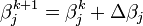
k is an iteration number and the vector of increments,  is known as the shift vector. At each iteration The model may be linearized by approximation to a first-order Taylor series expansion about

The Jacobian, J, is a function of constants, the independent variable and the parameters, so it changes from one iteration to the next. The residuals are given by

and the gradient equations become
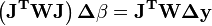
which, on rearrangement, become n simultaneous linear equations, the normal equations.
The normal equations are written in matrix notation as
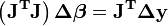
These are the defining equations of the Gauss-Newton algorithm.
Differences between linear and non-linear least squares
- The model function, f, in LLSQ (linear least squares) is a linear combination of parameters of the form
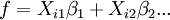 The model may represent a straight line, a parabola or any other polynomial-type function. In NLLSQ (Non-linear least squares) the parameters appear as functions, such as
  and so forth. If the derivatives
  are either constant or depend only on the values of the independent variable, the model is linear in the parameters. Otherwise the model is non-linear.
 - NLLSQ requires initial values for the parameters, LLSQ does not.
- NLLSQ requires that the Jacobian be calculated. Analytical expressions for the partial derivatives can be complicated. If analytical expressions are impossible to obtain the partial derivatives must be calculated by numerical approximation.
- In NLLSQ divergence is a common phenomenon whereas in LLSQ it is quite rare. Divergence occurs when the sum of squares increases from one iteration to the next. It is caused by the inadequacy of the approximation that the Taylor series can be truncated at the first term. When divergence occurs the method must be modified. The Levenberg-Marquardt algorithm provides good protection against divergence by rotating the shift vector towards the direction of steepest descent. By definition convergence is assured when the shift vector points in the direction of steepest descent.
- NLLSQ is an inherently iterative process.The iterative process has to be terminated when a convergence criterion is satisfied. LLSQ solutions can be computed using direct methods, although problems with large numbers of parameters are typically solved with iterative methods, such as the Gauss-Seidel method..
- In LLSQ the solution is unique, but in NLLSQ there may be multiple minima in the sum of squares.
- In NLLSQ estimates of the parameter errors are biased, but in LLSQ they are not.
These differences must be considered whenever the solution to a non-linear least squares problem is being sought.
Least squares, regression analysis and statistics
The methods of least squares and Regression analysis may appear to be different methods, but there are substantial similarities between them which are obscured by the use of different languages used to describe the methods. Both methods are used to model data obtained from observations, and both may use the same numerical techniques.
In the physical sciences the model usually has a theoretical basis. For example, a spring should obey Hooke's law which states that the extension of a spring is proportional to the force, F, applied to it.
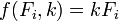
constitutes the model, where F is the independent variable. To determine the force constant, k, a series of measurements with different forces will produce a set of data, 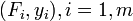 , where yi is a measured spring extension. The sum of squares to be minimized is
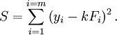
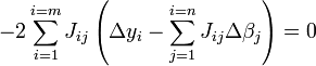
The least squares estimate of the force constant, k, is given by
Here it is assumed that application of the force causes the spring to expand and, having derived the force constant by least squares fitting, the extension can be predicted from Hooke's law.
In regression analysis the model is often an empirical one. For example, a very common model is the straight line model which is used to test if there is a linear relationship between dependent and independent variable. If a linear relationship is found to exist, the variables are said to be correlated. However it is well known that correlation does not prove causation, as both variables may be correlated with other, hidden, variables. For example, there is a correlation between deaths by drowning and the volume of ice cream sales. Both the number of people going swimming and the volume of ice cream sales increase as the weather gets hotter and it can be assumed that the number of deaths by drowning correlates with the number of people going swimming.
In both methods it is usually assumed that the independent variable is free from error, but that the dependent variable is subject to experimental error,  .
.
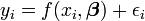
In this expression the model value is assumed to approximate to the true value, that is, the value that would be observed if there were no error. It is assumed that the experimental error ε is a random variable with mean zero, that is, it excludes all errors of a systematic nature. Since the model is only an approximation to the true value, the residuals are conceptually different from the errors. If the independent variable is subject to error, total least squares must be used.
In order to make statistical tests on the results it is necessary to make assumptions about the nature of the experimental errors. The most common assumption is that the errors belong to a Normal distribution. The central limit theorem supports the idea that this is a good assumption in many cases.
- The Gauss-Markov theorem. In a linear model in which the errors have expectation zero, are uncorrelated and have equal variances, the best linear unbiased estimator of any linear combination of the observations, is its least-squares estimator. "Best" means that the least squares estimators of the parameters have minimum variance. The assumption of equal variance is valid when the errors all belong to the same distribution.
- In a linear model, if the errors belong to a Normal distribution the least squares estimators are also the maximum likelihood estimators.
The assumption that the errors belong to a particular distribution function is not confined to regression analysis. Indeed, such assumptions must be made when making statistical tests on the parameters. In a least squares calculation with unit weights, or in linear regression, the variance on the jth parameter is given by
![\sigma^2(\beta_j)=\frac{S}{m-n}\left( \left[X^TX\right]^{-1}\right)_{jj}.](../../images/203/20359.png)
Confidence limits can be found if the probability distribution of the parameters is known, or assumed. Likewise statistical tests on the residuals can be made if the probability distribution of the residuals is known or assumed. The probability distribution of any linear combination of the dependent variables can be derived if the probability distribution of experimental errors is known or assumed. Most commonly it is assumed that experimental errors belong to a Normal distribution. In that case, it is often assumed that the parameters and residuals belong to a Student's t-distribution.
The sum of squared residuals can be expressed as

The matrix 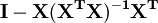 is a symmetric idempotent matrix of rank m-n. Here is an example of the use of that fact in the theory of linear regression. The eigenvalues of an idempotent matrix are either 0 or 1. Therefore m-n eigenvalues this matrix are equal to 1 and n eigenvalues are equal to zero. That is most of the work in showing that the sum of squared residuals has a chi-square distribution with m-n degrees of freedom.
Weighted least squares
The expressions given above are based on the implicit assumption that all the measurements are uncorrelated and have equal uncertainty. The Gauss-Markov theorem shows that, when this is so, is a best linear unbiased estimator (BLUE). If, however, the measurements are uncorrelated but have different uncertainties, a modified approach must be adopted. Aitken showed that when a weighted sum of squared residuals is minimized, is BLUE if each weight is equal to the reciprocal of the variance of the measurement.
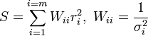
The gradient equations for this sum of squares are
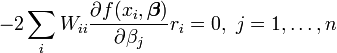
which, in a linear least squares system give the modified normal equations
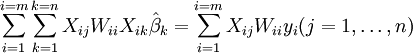
or
When the observational errors are uncorrelated the weight matrix, W, is diagonal. If the errors are correlated, the weight matrix should be equal to the inverse of the variance-covariance matrix of the observations, but this does not affect the matrix expression of the normal equations and the parameter estimates are still BLUE. See Generalized least squares for more details.
When the errors are uncorrelated, it is convenient to simplify the calculations to factor the weight matrix as  . The normal equations can then be written as

For non-linear least squares systems a similar argument shows that the normal equations should be modified as follows.
Other methods
Least squares estimation for linear models is notoriously non-robust to outliers. If the distribution of the outliers is skewed, the estimates can be biased. In the presence of any outliers, the least squares estimates are inefficient and can be extremely slow. When outliers occur in the data, methods of robust regression are more appropriate.
The technique of partial least squares is gaining popularity in chemometrics and other disciplines. It is used when the model is partially known and partially unknown.
Regression parameters can also be estimated by Bayesian methods. This has the advantages that
- confidence intervals can be produced for parameter estimates without the use of asymptotic approximations,
- prior information can be incorporated into the analysis.
In the linear regression,
suppose that we know from domain knowledge that can only take one of the values {−1, +1} but we do not know which. We can build this information into the analysis by choosing a prior for which is a discrete distribution with a probability of 0.5 on −1 and 0.5 on +1. The posterior for will also be a discrete distribution on {−1, +1}, but the probability weights will change to reflect the evidence from the data.
Lasso method
In some contexts a regularized version of the least squares solution may be preferable. The LASSO algorithm, for example, finds a least-squares solution with the constraint that  , the L1-norm of the parameter vector, is no greater than a given value. Equivalently, it may solve an unconstrained minimization of the least-squares penalty with
  added, where is a constant. (This is the Lagrangian dual of the constrained problem.) This problem may be solved using quadratic programming or more general convex optimization methods. The L1-regularized formulation is useful in some contexts due to its tendency to prefer solutions with fewer nonzero parameter values, effectively reducing the number of variables upon which the given solution is dependent .