Linear equation

Related subjects: Mathematics

About this schools Wikipedia selection

This Wikipedia selection is available offline from SOS Children for distribution in the developing world. A quick link for child sponsorship is http://www.sponsor-a-child.org.uk/

Graph sample of linear equations

A linear equation is an algebraic equation in which each term is either a constant or the product of a constant times the first power of a variable. Such an equation is equivalent to equating a first-degree polynomial to zero. These equations are called "linear" because they represent straight lines in Cartesian coordinates. A common form of a linear equation in the two variables $x$ and $y$ is

$y = mx + b.\,$

In this form, the constant $m$ will determine the slope or gradient of the line; and the constant term $b$ will determine the point at which the line crosses the y-axis. Equations involving terms such as x², y^1/3, and xy are nonlinear.

Forms for 2D linear equations

Complicated linear equations, such as the ones above, can be rewritten using the laws of elementary algebra into several simpler forms. In what follows x, y and t are variables; other letters represent constants (unspecified but fixed numbers).

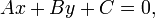
General form

$Ax + By + C = 0,\,$

where A and B are not both equal to zero. The equation is usually written so that A ≥ 0, by convention. The graph of the equation is a straight line, and every straight line can be represented by an equation in the above form. If A is nonzero, then the x-intercept, that is the x- coordinate of the point where the graph crosses the x-axis (y is zero), is −C/A. If B is nonzero, then the y-intercept, that is the y-coordinate of the point where the graph crosses the y-axis (x is zero), is −C/B, and the slope of the line is −A/B.

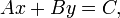
Standard form

$Ax + By = C,\,$

where A, B, and C are integers whose greatest common factor is 1, A and B are not both equal to zero and, A is non-negative (and if A=0 then B has to be positive). The standard form can be converted to the general form, but not always to all the other forms if A or B is zero.

Slope–intercept form

Y-axis formula

$y = mx + b,\,$

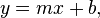
where m is the slope of the line and b is the y-intercept, which is the y-coordinate of the point where the line crosses the y axis. This can be seen by letting $x = 0$ , which immediately gives $y = b$ .

X-axis formula

$x = \frac{y}{m} + c,\,$

where m is the slope of the line and c is the x-intercept, which is the x-coordinate of the point where the line crosses the x axis. This can be seen by letting $y = 0$ , which immediately gives $x = c$ .

Point–slope form

$y - y_1 = m \cdot ( x - x_1 ),$

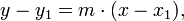
where m is the slope of the line and (x₁,y₁) is any point on the line. The point-slope and slope-intercept forms are easily interchangeable.

The point-slope form expresses the fact that the difference in the y coordinate between two points on a line (that is, $y - y_1$ ) is proportional to the difference in the x coordinate (that is, $x - x_1$ ). The proportionality constant is m (the slope of the line).

Intercept form

$\frac{x}{c} + \frac{y}{b} = 1$

where c and b must be nonzero. The graph of the equation has x-intercept c and y-intercept b. The intercept form can be converted to the standard form by setting A = 1/c, B = 1/b and C = 1.

Two-point form

$y - k = \frac{q - k}{p - h} (x - h),$

where p ≠ h. The graph passes through the points (h,k) and (p,q), and has slope m = (q−k) / (p−h).

Parametric form

$x = T t + U\,$

and

$y = V t + W.\,$

Two simultaneous equations in terms of a variable parameter t, with slope m = V / T, x-intercept (VU−WT) / V and y-intercept (WT−VU) / T.

This can also be related to the two-point form, where T = p−h, U = h, V = q−k, and W = k:

$x = (p - h) t + h\,$

and

$y = (q - k)t + k.\,$

In this case t varies from 0 at point (h,k) to 1 at point (p,q), with values of t between 0 and 1 providing interpolation and other values of t providing extrapolation.

Normal form

$y \sin \phi + x \cos \phi - p = 0,\,$

where φ is the angle of inclination of the normal and p is the length of the normal. The normal is defined to be the shortest segment between the line in question and the origin. Normal form can be derived from general form by dividing all of the coefficients by $\frac{|C|}{-C}\sqrt{A^2 + B^2}$ . This form also called Hesse standard form, named after a German mathematician Ludwig Otto Hesse.

Special cases

$y = b.\,$

This is a special case of the standard form where A = 0 and B = 1, or of the slope-intercept form where the slope M = 0. The graph is a horizontal line with y-intercept equal to b. There is no x-intercept, unless b = 0, in which case the graph of the line is the x-axis, and so every real number is an x-intercept.

$x = c.\,$

This is a special case of the standard form where A = 1 and B = 0. The graph is a vertical line with x-intercept equal to c. The slope is undefined. There is no y-intercept, unless c = 0, in which case the graph of the line is the y-axis, and so every real number is a y-intercept.

$y = y \$ and $x = x.\,$

In this case all variables and constants have canceled out, leaving a trivially true statement. The original equation, therefore, would be called an identity and one would not normally consider its graph (it would be the entire xy-plane). An example is 2x + 4y = 2(x + 2y). The two expressions on either side of the equal sign are always equal, no matter what values are used for x and y.

$e = f.\,$

In situations where algebraic manipulation leads to a statement such as 1 = 0, then the original equation is called inconsistent, meaning it is untrue for any values of x and y (i.e. its graph would be the empty set) An example would be 3x + 2 = 3x − 5.

Connection with linear functions and operators

In all of the named forms above (assuming the graph is not a vertical line), the variable y is a function of x, and the graph of this function is the graph of the equation.

In the particular case that the line crosses through the origin, if the linear equation is written in the form y = f(x) then f has the properties:

$f ( x + y ) = f ( x ) + f ( y )\,$

and

$f ( a x ) = a f ( x ),\,$

where a is any scalar. A function which satisfies these properties is called a linear function, or more generally a linear map. This property makes linear equations particularly easy to solve and reason about.

Linear equations occur with great regularity in applied mathematics. While they arise quite naturally when modeling many phenomena, they are particularly useful since many non-linear equations may be reduced to linear equations by assuming that quantities of interest vary to only a small extent from some "background" state.

Linear equations in more than two variables

A linear equation can involve more than two variables. The general linear equation in n variables is:

$a_1 x_1 + a_2 x_2 + \cdots + a_n x_n = b.$

In this form, a₁, a₂, …, a_n are the coefficients, x₁, x₂, …, x_n are the variables, and b is the constant. When dealing with three or fewer variables, it is common to replace x₁ with just x, x₂ with y, and x₃ with z, as appropriate.

Such an equation will represent an (n–1)-dimensional hyperplane in n-dimensional Euclidean space (for example, a plane in 3-space).

Retrieved from " http://en.wikipedia.org/w/index.php?title=Linear_equation&oldid=198721570"

We provide Linux to the World