

Linear regression
About this schools Wikipedia selection
SOS Children offer a complete download of this selection for schools for use on schools intranets. Before you decide about sponsoring a child, why not learn about different sponsorship charities first?
Linear regression is a form of regression analysis in which observational data are modeled by a least squares function which is a linear combination of the model parameters and depends on one or more independent variables. In simple linear regression the model function represents a straight line. The results of data fitting are subject to statistical analysis.

Definitions
The data consist of m values  taken from observations of the dependent variable ( response variable)
  . The dependent variable is subject to error. This error is assumed to be random variable, with a mean of zero. Systematic error (e.g. mean ≠ 0) may be present but its treatment is outside the scope of regression analysis. The independent variable ( explanatory variable)
  , is error-free. If this is not so, modeling should be done using errors-in-variables model techniques. The independent variables are also called regressors, exogenous variables, input variables and predictor variables. In simple linear regression the data model is written as
where  is an observational error.
  (intercept) and
  (slope) are the parameters of the model. In general there are n parameters,
  and the model can be written as
where the coefficients  are constants or functions of the independent variable, x. Models which do not conform to this specification must be treated by nonlinear regression.
Unless otherwise stated it is assumed that the observational errors are uncorrelated and belong to a normal distribution. This, or another assumption, is used when performing statistical tests on the regression results. An equivalent formulation of simple linear regression that explicitly shows the linear regression as a model of conditional expectation can be given as
The conditional distribution of y given x is a linear transformation of the distribution of the error term.
Notation and naming conventions
- Scalars and vectors are denoted by lower case letters.
- Matrices are denoted by upper case letters.
- Parameters are denoted by Greek letters.
- Vectors and matrices are denoted by bold letters.
- A parameter with a hat, such as
 , denotes a parameter estimator.
Least-squares analysis
The first objective of regression analysis is to best-fit the data by adjusting the parameters of the model. Of the different criteria that can be used to define what constitutes a best fit, the least squares criterion is a very powerful one. The objective function, S, is defined as a sum of squared residuals, ri

where each residual is the difference between the observed value and the value calculated by the model:
The best fit is obtained when S, the sum of squared residuals, is minimized. Subject to certain conditions, the parameters then have minimum variance ( Gauss-Markov theorem) and may also represent a maximum likelihood solution to the optimization problem.
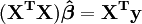
From the theory of linear least squares, the parameter estimators are found by solving the normal equations
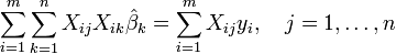
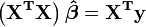
In matrix notation, these equations are written as
 ,
,
And thus when the matrix  is non singular:
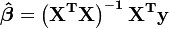 ,
,
Specifically, for straight-line fitting, this is shown in straight line fitting.
Regression statistics
The second objective of regression is the statistical analysis of the results of data fitting.
Denote by  the variance of the error term
  (so that
 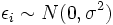 for every
  ). An unbiased estimate of is given by
 .
.
The relation between the estimate and the true value is:
where  has Chi-square distribution with
  degrees of freedom.
Application of this test requires that , the variance of an observation of unit weight, be estimated. If the  test is passed, the data may be said to be fitted within observational error.
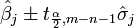
The solution to the normal equations can be written as
This shows that the parameter estimators are linear combinations of the dependent variable. It follows that, if the observational errors are normally distributed, the parameter estimators will belong to a Student's t distribution with degrees of freedom. The standard deviation on a parameter estimator is given by
![\hat\sigma_j=\sqrt{ \frac{S}{m-n}\left[\mathbf{(X^TX)}^{-1}\right]_{jj}}](../../images/216/21697.png)
The 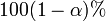 confidence interval for the parameter,
  , is computed as follows:
The residuals can be expressed as

The matrix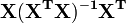 is known as the hat matrix and has the useful property that it is idempotent. Using this property it can be shown that, if the errors are normally distributed, the residuals will follow a Student's t distribution with degrees of freedom. Studentized residuals are useful in testing for outliers.
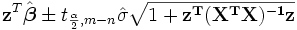
Given a value of the independent variable, xd, the predicted response is calculated as
Writing the elements  as
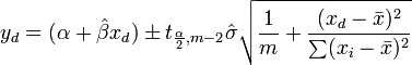
as  , the mean response confidence interval for the prediction is given, using error propagation theory, by:
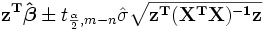
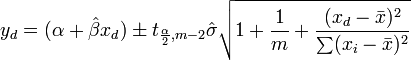
The predicted response confidence intervals for the data are given by:
 .
.
Linear case
In the case that the formula to be fitted is a straight line,  , the normal equations are
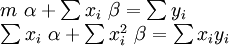
where all summations are from i=1 to i=m. Thence, by Cramer's rule,
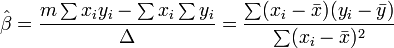
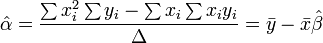
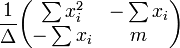
where
The covariance matrix is
The mean response confidence interval is given by
The predicted response confidence interval is given by
Variance analysis
Variance analysis is similar to ANOVA in that the sum of squared residuals is split into two components. The regression sum of squares (or sum of squared residuals) SSR (also commonly called RSS) is given by:
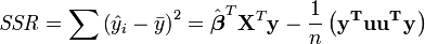
where  and u is an n by 1 unit vector (i.e. each element is 1). Note that the terms
  and
and  are both equivalent to
  , and so the term
  is equivalent to
  .
.
The error (or unexplained) sum of squares ESS is given by:

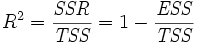
The total sum of squares TSS is given by

Pearson's coefficient of regression, R² is then given as
Example
To illustrate the various goals of regression, we give an example. The following data set gives the average heights and weights for American women aged 30-39 (source: The World Almanac and Book of Facts, 1975).
-
Height/ m 1.47 1.5 1.52 1.55 1.57 1.60 1.63 1.65 1.68 1.7 1.73 1.75 1.78 1.8 1.83 Weight/kg 52.21 53.12 54.48 55.84 57.2 58.57 59.93 61.29 63.11 64.47 66.28 68.1 69.92 72.19 74.46
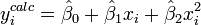
A plot of weight against height (see below) shows that it cannot be modeled by a straight line, so a regression is performed by modeling the data by a parabola.
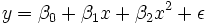
where the dependent variable, y, is weight and the independent variable, x is height.
Place the coefficients,  , of the parameters for the ith observation in the ith row of the matrix X.


The values of the parameters are found by solving the normal equations
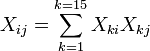
Element ij of the normal equation matrix,  is formed by summing the products of column i and column j of X.
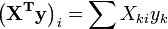
Element i of the right-hand side vector  is formed by summing the products of column i of X with the column of independent variable values.
Thus, the normal equations are
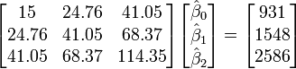
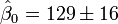 (value
  standard deviation)
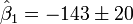

The calculated values are given by
The observed and calculated data are plotted together and the residuals,  , are calculated and plotted. Standard deviations are calculated using the sum of squares,
  .
.
The confidence intervals are computed using:
![[\hat{\beta_j}-\sigma_j t_{m-n;1-\frac{\alpha}{2}};\hat{\beta_j}+\sigma_j t_{m-n;1-\frac{\alpha}{2}}]](../../images/217/21747.png)
with  =5%,
=5%,  = 2.2. Therefore, we can say that the 95% confidence intervals are:
![\beta_0\in[92.9,164.7]](../../images/217/21749.png)
![\beta_1\in[-186.8,-99.5]](../../images/217/21750.png)
![\beta_2\in[48.7,75.2]](../../images/217/21751.png)
Checking model assumptions
The model assumptions are checked by calculating the residuals and plotting them. The following plots can be constructed to test the validity of the assumptions:
- Residuals against the explanatory variable, as illustrated above.
- A time series plot of the residuals, that is, plotting the residuals as a function of time.
- Residuals against the fitted values,
 .
. - Residuals against the preceding residual.
- A normal probability plot of the residuals to test normality. The points should lie along a straight line.
There should not be any noticeable pattern to the data in all but the last plot
Checking model validity
The validity of the model can be checked using any of the following methods:
- Using the confidence interval for each of the parameters, . If the confidence interval includes 0, then the parameter can be removed from the model. Ideally, a new regression analysis excluding that parameter would need to be performed and continued until there are no more parameters to remove.
- When fitting a straight line, calculate Pearson’s coefficient of regression. The closer the value is to 1; the better the regression is. This coefficient gives what fraction of the observed behaviour can be explained by the given variables.
- Examining the observational and prediction confidence intervals. The smaller they are the better.
- Computing the F-statistics.
Other procedures
Weighted least squares
Weighted least squares is a generalisation of the least squares method, used when the observational errors have unequal variance.
Errors-in-variables model
Errors-in-variables model or total least squares when the independent variable is subject to error
Generalized linear model
Generalized linear model is used when the distribution function of the errors is not a Normal distribution. Examples include Exponential distribution, gamma distribution, Inverse Gaussian distribution, Poisson distribution, binomial distribution, multinomial distribution
Robust regression
A host of alternative approaches to the computation of regression parameters are included in the category known as robust regression. One technique minimizes the mean absolute error, or some other function of the residuals, instead of mean squared error as in linear regression. Robust regression is much more computationally intensive than linear regression and is somewhat more difficult to implement as well. While least squares estimates are not very sensitive to breaking the normality of the errors assumption, this is not true when the variance or mean of the error distribution is not bounded, or when an analyst that can identify outliers is unavailable.
Among Stata users, Robust regression is frequently taken to mean linear regression with Huber-White standard error estimates due to the naming conventions for regression commands. This procedure relaxes the assumption of homoscedasticity for variance estimates only; the predictors are still ordinary least squares (OLS) estimates. This occasionally leads to confusion; Stata users sometimes believe that linear regression is a robust method when this option is used, although it is actually not robust in the sense of outlier-resistance.
Applications of linear regression
Linear regression is widely used in biological, behavioural and social sciences to describe relationships between variables. It ranks as one of the most important tools used in these disciplines.
The trend line
A trend line represents a trend, the long-term movement in time series data after other components have been accounted for. It tells whether a particular data set (say GDP, oil prices or stock prices) have increased or decreased over the period of time. A trend line could simply be drawn by eye through a set of data points, but more properly their position and slope is calculated using statistical techniques like linear regression. Trend lines typically are straight lines, although some variations use higher degree polynomials depending on the degree of curvature desired in the line.
Trend lines are sometimes used in business analytics to show changes in data over time. This has the advantage of being simple. Trend lines are often used to argue that a particular action or event (such as training, or an advertising campaign) caused observed changes at a point in time. This is a simple technique, and does not require a control group, experimental design, or a sophisticated analysis technique. However, it suffers from a lack of scientific validity in cases where other potential changes can affect the data.
Medicine
As one example, early evidence relating tobacco smoking to mortality and morbidity came from studies employing regression. Researchers usually include several variables in their regression analysis in an effort to remove factors that might produce spurious correlations. For the cigarette smoking example, researchers might include socio-economic status in addition to smoking to ensure that any observed effect of smoking on mortality is not due to some effect of education or income. However, it is never possible to include all possible confounding variables in a study employing regression. For the smoking example, a hypothetical gene might increase mortality and also cause people to smoke more. For this reason, randomized controlled trials are considered to be more trustworthy than a regression analysis.
Finance
The capital asset pricing model uses linear regression as well as the concept of Beta for analyzing and quantifying the systematic risk of an investment. This comes directly from the Beta coefficient of the linear regression model that relates the return on the investment to the return on all risky assets.
Regression may not be the appropriate way to estimate beta in finance given that it is supposed to provide the volatility of an investment relative to the volatility of the market as a whole. This would require that both these variables be treated in the same way when estimating the slope. Whereas regression treats all variability as being in the investment returns variable, i.e. it only considers residuals in the dependent variable.