

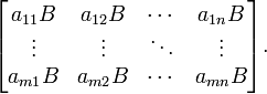
Matrix multiplication
Background to the schools Wikipedia
SOS Children volunteers helped choose articles and made other curriculum material A good way to help other children is by sponsoring a child
In mathematics, matrix multiplication is the operation of multiplying a matrix with either a scalar or another matrix. This article gives an overview of the various ways to perform matrix multiplication.
Ordinary matrix product
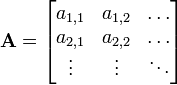
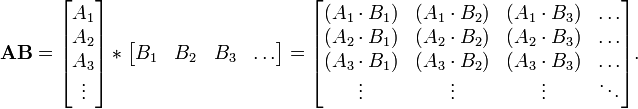
This is the most often used and most important way to multiply matrices. It is defined between two matrices only if the number of columns of the first matrix is the same as the number of rows of the second matrix. If A is an m-by-n matrix and B is an n-by-p matrix, then their product is an m-by-p matrix denoted by AB (or sometimes A · B). If C = AB, and ci,j denotes the entry in C at position (i,j), then
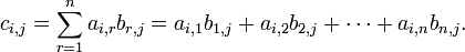
for each pair i and j with 1 ≤ i ≤ m and 1 ≤ j ≤ p. The algebraic system of " matrix units" summarises the abstract properties of this kind of multiplication.
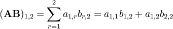
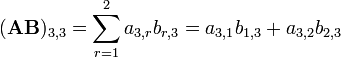
Calculating directly from the definition

The picture to the left shows how to calculate the (1,2) element and the (3,3) element of AB if A is a 4×2 matrix, and B is a 2×3 matrix. Elements from each matrix are paired off in the direction of the arrows; each pair is multiplied and the products are added. The location of the resulting number in AB corresponds to the row and column that were considered.
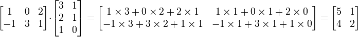
For example:
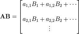
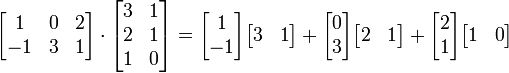
The coefficients-vectors method
This matrix multiplication can also be considered from a slightly different viewpoint: it adds vectors together after being multiplied by different coefficients. If A and B are matrices given by:
 and
and 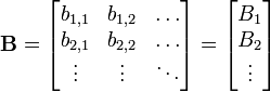
then
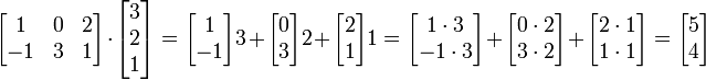
The example revisited:


The rows in the matrix on the left are the list of coefficients. The matrix on the right is the list of vectors. In the example, the first row is [1 0 2], and thus we take 1 times the first vector, 0 times the second vector, and 2 times the third vector.
The equation can be simplified further by using outer products:
The terms of this sum are matrices of the same shape, each describing the effect of one column of A and one row of B on the result. The columns of A can be seen as a coordinate system of the transform, i.e. given a vector x we have  where
where  are coordinates along the
  "axes". The terms
  are like
  , except that
  contains the ith coordinate for each column vector of B, each of which is transformed independently in parallel.
The example revisited:

The vectors  and
and  have been transformed to
  and
and  in parallel. One could also transform them one by one with the same steps:
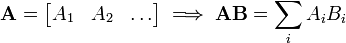
Vector-lists method
The ordinary matrix product can be thought of as a dot product of a column-list of vectors and a row-list of vectors. If A and B are matrices given by:
 and
and 
where
- A1 is the row vector of all elements of the form a1,x A2 is the row vector of all elements of the form a2,x etc,
- and B1 is the column vector of all elements of the form bx,1 B2 is the column vector of all elements of the form bx,2 etc,
then
Properties
Matrix multiplication is not commutative (that is, AB ≠ BA), except in special cases. It is easy to see why: you cannot expect to switch the proportions with the vectors and get the same result. It is also easy to see how the order of the factors determines the result when one knows that the number of columns in the proportions matrix has to be the same as the number of rows in the vectors matrix: they have to represent the same number of vectors.
Although matrix multiplication is not commutative, the determinants of AB and BA are always equal (if A and B are square matrices of the same size). See the article on determinants for an explanation. However matrix multiplication is commutative when both matrices are diagonal and of the same dimension.
This notion of multiplication is important because if A and B are interpreted as linear transformations (which is almost universally done), then the matrix product AB corresponds to the composition of the two linear transformations, with B being applied first.
Additionally, all notions of matrix multiplication described here share a set of common properties described below.
Algorithms
The complexity of matrix multiplication, if carried out naively, is O(n³), but more efficient algorithms do exist. Strassen's algorithm, devised by Volker Strassen in 1969 and often referred to as "fast matrix multiplication", is based on a clever way of multiplying two 2 × 2 matrices which requires only 7 multiplications (instead of the usual 8). Applying this trick recursively gives an algorithm with a cost of 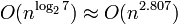 . In practice, though, it is rarely used since it is awkward to implement and it lacks numerical stability. The constant factor implied in the big O notation is about 4.695.
The algorithm with the lowest known exponent, which was presented by Don Coppersmith and Shmuel Winograd in 1990, has an asymptotic complexity of O(n2.376). It is similar to Strassen's algorithm: a clever way is devised for multiplying two k × k matrices with fewer than k³ multiplications, and this technique is applied recursively. It improves on the constant factor in Strassen's algorithm, reducing it to 4.537. However, the constant term implied in the O(n2.376) result is so large that the Coppersmith–Winograd algorithm is only worthwhile for matrices that are too big to handle on present-day computers (Knuth, 1998).
Since any algorithm for multiplying two n × n matrices has to process all 2 × n² entries, there is an asymptotic lower bound of Ω(n²) operations. Raz (2002) proves a lower bound of 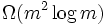 for bounded coefficient arithmetic circuits over the real or complex numbers.
Cohn et al. (2003, 2005) put methods such as the Strassen and Coppersmith–Winograd algorithms in an entirely different, group-theoretic context. They show that if families of wreath products of Abelian with symmetric groups satisfying certain conditions exists, matrix multiplication algorithms with essential quadratic complexity exist. Most researchers believe that this is indeed the case (Robinson, 2005).
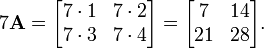
Scalar multiplication
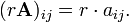
The scalar multiplication of a matrix A = (aij) and a scalar r gives a product r A of the same size as A. The entries of r A are given by
For example, if

then
If we are concerned with matrices over a ring, then the above multiplication is sometimes called the left multiplication while the right multiplication is defined to be
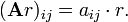
When the underlying ring is commutative, for example, the real or complex number field, the two multiplications are the same. However, if the ring is not commutative, such as the quaternions, they may be different. For example
Hadamard product
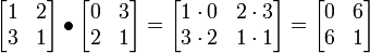
For two matrices of the same dimensions, we have the Hadamard product, also known as the entrywise product and the Schur product. It can be generalized to hold not only for matrices but also for operators. The Hadamard product of two m-by-n matrices A and B, denoted by A • B, is an m-by-n matrix given by (A•B)ij = aij bij. For instance
 .
.
Note that the Hadamard product is a submatrix of the Kronecker product (see below).
The Hadamard product is commutative.
The Hadamard product is studied by matrix theorists, and it appears in lossy compression algorithms such as JPEG, but it is virtually untouched by linear algebraists. It is discussed in (Horn & Johnson, 1994, Ch. 5).
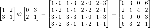
Kronecker product
For any two arbitrary matrices A and B, we have the direct product or Kronecker product A ⊗ B defined as
Note that if A is m-by-n and B is p-by-r then A ⊗ B is an mp-by-nr matrix. Again this multiplication is not commutative.
For example
 .
.
If A and B represent linear transformations V1 → W1 and V2 → W2, respectively, then A ⊗ B represents the tensor product of the two maps, V1 ⊗ V2 → W1 ⊗ W2.
Common properties
| The Wikibook The Book of Mathematical Proofs has a page on the topic of: Proofs of properties of matrices |
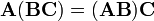
All three notions of matrix multiplication are associative:
and distributive:
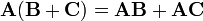
and
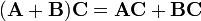 .
.
and compatible with scalar multiplication:
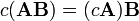
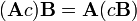
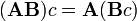
Note that these three separate couples of expressions will be equal to each other only if the multiplication and addition on the scalar field are commutative, i.e. the scalar field is a commutative ring. See Scalar multiplication above for a counter-example such as the scalar field of quaternions.
Frobenius inner product
The Frobenius inner product, sometimes denoted A:B is the component-wise inner product of two matrices as though they are vectors. In other words, it is the sum of the entries of the Hadamard product, that is,
This inner product induces the Frobenius norm.