Student's t-distribution

Related subjects: Mathematics

Background Information

This wikipedia selection has been chosen by volunteers helping SOS Children from Wikipedia for this Wikipedia Selection for schools. See http://www.soschildren.org/sponsor-a-child to find out about child sponsorship.

Student's t
Probability density function
Cumulative distribution function
Parameters	$\nu > 0$ degrees of freedom (real)
Support	$x \in (-\infty; +\infty)\!$
PDF	$\frac{\Gamma(\frac{\nu+1}{2})} {\sqrt{\nu\pi}\,\Gamma(\frac{\nu}{2})} \left(1+\frac{x^2}{\nu} \right)^{-(\frac{\nu+1}{2})}\!$
CDF	$\begin{matrix} \frac{1}{2} + x \Gamma \left( \frac{\nu+1}{2} \right) \cdot\\[0.5em] \frac{\,_2F_1 \left ( \frac{1}{2},\frac{\nu+1}{2};\frac{3}{2}; -\frac{x^2}{\nu} \right)} {\sqrt{\pi\nu}\,\Gamma (\frac{\nu}{2})} \end{matrix}$ where $\,_2F_1$ is the hypergeometric function
Mean	$0\text{ for }\nu>1$ , otherwise undefined
Median	$0$
Mode	$0$
Variance	$\frac{\nu}{\nu-2}\text{ for }\nu>2\!$ , otherwise undefined
Skewness	$0\text{ for }\nu>3$
Ex. kurtosis	$\frac{6}{\nu-4}\text{ for }\nu>4\!$
Entropy	$\begin{matrix} \frac{\nu+1}{2}\left[ \psi(\frac{1+\nu}{2}) - \psi(\frac{\nu}{2}) \right] \\[0.5em] + \log{\left[\sqrt{\nu}B(\frac{\nu}{2},\frac{1}{2})\right]} \end{matrix}$ $\psi$ : digamma function, $B$ : beta function
MGF	(Not defined)

The Student's t-distribution (or also t-distribution), in probability and statistics, is a probability distribution that arises in the problem of estimating the mean of a normally distributed population when the sample size is small. It is the basis of the popular Student's t-tests for the statistical significance of the difference between two sample means, and for confidence intervals for the difference between two population means. The Student's t-distribution is a special case of the generalised hyperbolic distribution.

The derivation of the t-distribution was first published in 1908 by William Sealy Gosset, while he worked at a Guinness Brewery in Dublin. He was prohibited from publishing under his own name, so the paper was written under the pseudonym Student. The t-test and the associated theory became well-known through the work of R.A. Fisher, who called the distribution "Student's distribution".

Student's distribution arises when (as in nearly all practical statistical work) the population standard deviation is unknown and has to be estimated from the data. Textbook problems treating the standard deviation as if it were known are of two kinds: (1) those in which the sample size is so large that one may treat a data-based estimate of the variance as if it were certain, and (2) those that illustrate mathematical reasoning, in which the problem of estimating the standard deviation is temporarily ignored because that is not the point that the author or instructor is then explaining.

Why use the Student's t-distribution

Confidence intervals and hypothesis tests rely on Student's t-distribution to cope with uncertainty resulting from estimating the standard deviation from a sample, whereas if the population standard deviation were known, a normal distribution would be used.

How Student's t-distribution comes about

Suppose X₁, ..., X_n are independent random variables that are normally distributed with expected value μ and variance σ². Let

$\overline{X}_n = (X_1+\cdots+X_n)/n$

be the sample mean, and

${S_n}^2=\frac{1}{n-1}\sum_{i=1}^n\left(X_i-\overline{X}_n\right)^2$

be the sample variance. It is readily shown that the quantity

$Z=\frac{\overline{X}_n-\mu}{\sigma/\sqrt{n}}$

is normally distributed with mean 0 and variance 1, since the sample mean $\scriptstyle \overline{X}_n$ is normally distributed with mean $\mu$ and standard error $\scriptstyle\sigma/\sqrt{n}$ .

Gosset studied a related pivotal quantity,

$T=\frac{\overline{X}_n-\mu}{S_n / \sqrt{n}},$

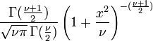
which differs from Z in that the exact standard deviation $\scriptstyle \sigma$ is replaced by the random variable $\scriptstyle S_n$ . Technically, $\scriptstyle(n-1)S_n^2/\sigma^2$ has a $\scriptstyle\chi_{n-1}^2$ distribution by Cochran's theorem. Gosset's work showed that T has the probability density function

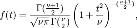
$f(t) = \frac{\Gamma(\frac{\nu+1}{2})} {\sqrt{\nu\pi}\,\Gamma(\frac{\nu}{2})} \left(1+\frac{t^2}{\nu} \right)^{-(\frac{\nu+1}{2})}\!,$

with ν equal to n − 1 and where Γ is the Gamma function.

This may also be written as

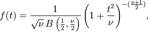
$f(t) = \frac{1}{\sqrt{\nu}\, B \left (\frac{1}{2}, \frac{\nu}{2}\right )} \left(1+\frac{t^2}{\nu} \right)^{-(\frac{\nu+1}{2})}\!,$

where B is the Beta function.

The distribution of T is now called the t-distribution. The parameter ν is called the number of degrees of freedom. The distribution depends on ν, but not μ or σ; the lack of dependence on μ and σ is what makes the t-distribution important in both theory and practice.

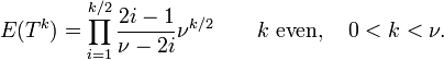
The moments of the t-distribution are

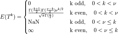
$E(T^k)=\begin{cases} 0 & \mbox{k odd},\quad 0<k< \nu\\ \frac{\Gamma(\frac{k+1}{2})\Gamma(\frac{\nu-k}{2})\nu^{k/2}}{\sqrt{\pi}\Gamma(\frac{\nu}{2})} & \mbox{k even}, \quad 0<k< \nu\\ \mbox{NaN} & \mbox{k odd},\quad 0<\nu\leq k\\ \infty & \mbox{k even},\quad 0<\nu\leq k\\ \end{cases}$

It should be noted that the term for 0 < k < ν, k even, may be simplified using the properties of the Gamma function to

$E(T^k)= \prod_{i=1}^{k/2} \frac{2i-1}{\nu - 2i}\nu^{k/2} \qquad k\mbox{ even},\quad 0<k<\nu.$

Confidence intervals derived from Student's t-distribution

Suppose the number A is so chosen that

$\Pr(-A < T < A)=0.9,\,$

when T has a t-distribution with n − 1 degrees of freedom. This is the same as

$\Pr(T < A) = 0.95,\,$

so A is the "95th percentile" of this probability distribution, or $A=t_{(0.05,n-1)}$ . Then

$\Pr \left (-A < {\overline{X}_n - \mu \over S_n/\sqrt{n}} < A \right)=0.9,$

and this is equivalent to

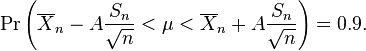
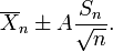
$\Pr\left(\overline{X}_n - A{S_n \over \sqrt{n}} < \mu < \overline{X}_n + A{S_n \over \sqrt{n}}\right) = 0.9.$

Therefore the interval whose endpoints are

$\overline{X}_n\pm A\frac{S_n}{\sqrt{n}}$

is a 90-percent confidence interval for μ. Therefore, if we find the mean of a set of observations that we can reasonably expect to have a normal distribution, we can use the t-distribution to examine whether the confidence limits on that mean include some theoretically predicted value - such as the value predicted on a null hypothesis.

It is this result that is used in the Student's t-tests: since the difference between the means of samples from two normal distributions is itself distributed normally, the t-distribution can be used to examine whether that difference can reasonably be supposed to be zero.

If the data are normally distributed, the one-sided (1 − a)-upper confidence limit (UCL) of the mean, can be calculated using the following equation:

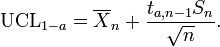
$\mathrm{UCL}_{1-a} = \overline{X}_n+\frac{t_{a,n-1} S_n}{\sqrt{n}}.$

The resulting UCL will be the greatest average value that will occur for a given confidence interval and population size. In other words, $\overline{X}_n$ being the mean of the set of observations, the probability that the mean of the distribution is inferior to $\mathrm{UCL}_{1-a}$ is equal to the confidence level $1-a.$

A number of other statistics can be shown to have t-distributions for samples of moderate size under null hypotheses that are of interest, so that the t-distribution forms the basis for significance tests in other situations as well as when examining the differences between means. For example, the distribution of Spearman's rank correlation coefficient, rho, in the null case (zero correlation) is well approximated by the t distribution for sample sizes above about 20.

See prediction interval for another example of the use of this distribution.

Integral of Student's probability density function and p-value

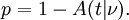
The function $\scriptstyle A(t|\nu)$ is the integral of Student's probability density function, ƒ(t) between −t and t. It thus gives the probability that a value of t less than that calculated from observed data would occur by chance. Therefore, the function $\scriptstyle A(t|\nu)$ can be used when testing whether the difference between the means of two sets of data is statistically significant, by calculating the corresponding value of t and the probability of its occurrence if the two sets of data were drawn from the same population. This is used in a variety of situations, particularly in t-tests. For the statistic t, with $\scriptstyle\nu$ degrees of freedom, $\scriptstyle A(t|\nu)$ is the probability that t would be less than the observed value if the two means were the same (provided that the smaller mean is subtracted from the larger, so that t > 0). It is defined for real t by the following formula:

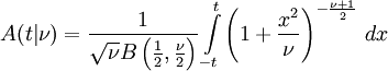
$A(t|\nu) = \frac{1}{\sqrt{\nu} B \left (\frac{1}{2}, \frac{\nu}{2}\right )} \int\limits_{-t}^{t} \left (1+\frac{x^2}{\nu}\right )^{-\frac{\nu +1}{2} }\, dx$

where B is the Beta function. For t > 0, there is a relation to the regularized incomplete beta function I_x(a, b) as follows:

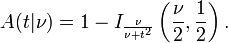
$A(t|\nu) = 1 - I_{\frac{\nu}{\nu +t^2}}\left(\frac{\nu}{2},\frac{1}{2}\right).$

The probability that a value of the t statistic greater than or equal to that observed would happen by chance, if the two sets of data were drawn from the same population, is given by

$p = {1-A(t|\nu)}.\,$

Further theory

Gosset's result can be stated more generally. (See, for example, Hogg and Craig, Sections 4.4 and 4.8.) Let Z have a normal distribution with mean 0 and variance 1. Let V have a chi-square distribution with ν degrees of freedom. Further suppose that Z and V are independent (see Cochran's theorem). Then the ratio

$\frac{Z}{\sqrt{V/\nu\ }}$

has a t-distribution with ν degrees of freedom.

For a t-distribution with ν degrees of freedom, the expected value is 0, and its variance is ν/(ν − 2) if ν > 2. The skewness is 0 and the kurtosis is 6/(ν − 4) if ν > 4.

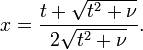
The cumulative distribution function is given by an incomplete beta function,

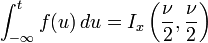
$\int_{-\infty}^t f(u)\,du = I_x\left(\frac{\nu}{2},\frac{\nu}{2}\right)$

with

$x = \frac{t+\sqrt{t^2+\nu}}{2\sqrt{t^2+\nu}}.$

The t-distribution is related to the F-distribution as follows: the square of a value of t with ν degrees of freedom is distributed as F with 1 and ν degrees of freedom.

The overall shape of the probability density function of the t-distribution resembles the bell shape of a normally distributed variable with mean 0 and variance 1, except that it is a bit lower and wider. As the number of degrees of freedom grows, the t-distribution approaches the normal distribution with mean 0 and variance 1.

The following images show the density of the t-distribution for increasing values of ν. The normal distribution is shown as a blue line for comparison.; Note that the t-distribution (red line) becomes closer to the normal distribution as ν increases. For ν = 30 the t-distribution is almost the same as the normal distribution.

Density of the t-distribution (red and green) for 1, 2, 3, 5, 10, and 30 df compared to normal distribution (blue)

Table of selected values

The following table lists a few selected values for t-distributions with ν degrees of freedom for a range of one-sided confidence intervals. For an example of how to read this table, take the fourth row, which begins with 4; that means ν, the number of degrees of freedom, is 4 (and if we are dealing, as above, with n values with a fixed sum, n = 5). Take the fifth entry, in the column headed 95%. The value of that entry is "2.132". Then the probability that T is less than 2.132 is 95% or $\mbox{Pr}\left( -\infty < T < 2.132\right) = 0.95$ ; the entry does not mean (as it might with other distributions) that $\mbox{Pr}\left( -2.132< T < 2.132\right) = 0.95$ .

In fact, by the symmetry of the distribution,

Pr(T < −2.132) = 1 − Pr(T > −2.132) = 1 − 0.95 = 0.05,

and so

Pr(−2.132 < T < 2.132) = 1 − 2(0.05) = 0.9.

Note that the last row also gives critical points: a t-distribution with infinitely-many degrees of freedom is a normal distribution. (See below: Related distributions).

$\nu$	75%	80%	85%	90%	95%	97.5%	99%	99.5%	99.75%	99.9%	99.95%
1	1.000	1.376	1.963	3.078	6.314	12.71	31.82	63.66	127.3	318.3	636.6
2	0.816	1.061	1.386	1.886	2.920	4.303	6.965	9.925	14.09	22.33	31.60
3	0.765	0.978	1.250	1.638	2.353	3.182	4.541	5.841	7.453	10.21	12.92
4	0.741	0.941	1.190	1.533	2.132	2.776	3.747	4.604	5.598	7.173	8.610
5	0.727	0.920	1.156	1.476	2.015	2.571	3.365	4.032	4.773	5.893	6.869
6	0.718	0.906	1.134	1.440	1.943	2.447	3.143	3.707	4.317	5.208	5.959
7	0.711	0.896	1.119	1.415	1.895	2.365	2.998	3.499	4.029	4.785	5.408
8	0.706	0.889	1.108	1.397	1.860	2.306	2.896	3.355	3.833	4.501	5.041
9	0.703	0.883	1.100	1.383	1.833	2.262	2.821	3.250	3.690	4.297	4.781
10	0.700	0.879	1.093	1.372	1.812	2.228	2.764	3.169	3.581	4.144	4.587
11	0.697	0.876	1.088	1.363	1.796	2.201	2.718	3.106	3.497	4.025	4.437
12	0.695	0.873	1.083	1.356	1.782	2.179	2.681	3.055	3.428	3.930	4.318
13	0.694	0.870	1.079	1.350	1.771	2.160	2.650	3.012	3.372	3.852	4.221
14	0.692	0.868	1.076	1.345	1.761	2.145	2.624	2.977	3.326	3.787	4.140
15	0.691	0.866	1.074	1.341	1.753	2.131	2.602	2.947	3.286	3.733	4.073
16	0.690	0.865	1.071	1.337	1.746	2.120	2.583	2.921	3.252	3.686	4.015
17	0.689	0.863	1.069	1.333	1.740	2.110	2.567	2.898	3.222	3.646	3.965
18	0.688	0.862	1.067	1.330	1.734	2.101	2.552	2.878	3.197	3.610	3.922
19	0.688	0.861	1.066	1.328	1.729	2.093	2.539	2.861	3.174	3.579	3.883
20	0.687	0.860	1.064	1.325	1.725	2.086	2.528	2.845	3.153	3.552	3.850
21	0.686	0.859	1.063	1.323	1.721	2.080	2.518	2.831	3.135	3.527	3.819
22	0.686	0.858	1.061	1.321	1.717	2.074	2.508	2.819	3.119	3.505	3.792
23	0.685	0.858	1.060	1.319	1.714	2.069	2.500	2.807	3.104	3.485	3.767
24	0.685	0.857	1.059	1.318	1.711	2.064	2.492	2.797	3.091	3.467	3.745
25	0.684	0.856	1.058	1.316	1.708	2.060	2.485	2.787	3.078	3.450	3.725
26	0.684	0.856	1.058	1.315	1.706	2.056	2.479	2.779	3.067	3.435	3.707
27	0.684	0.855	1.057	1.314	1.703	2.052	2.473	2.771	3.057	3.421	3.690
28	0.683	0.855	1.056	1.313	1.701	2.048	2.467	2.763	3.047	3.408	3.674
29	0.683	0.854	1.055	1.311	1.699	2.045	2.462	2.756	3.038	3.396	3.659
30	0.683	0.854	1.055	1.310	1.697	2.042	2.457	2.750	3.030	3.385	3.646
40	0.681	0.851	1.050	1.303	1.684	2.021	2.423	2.704	2.971	3.307	3.551
50	0.679	0.849	1.047	1.299	1.676	2.009	2.403	2.678	2.937	3.261	3.496
60	0.679	0.848	1.045	1.296	1.671	2.000	2.390	2.660	2.915	3.232	3.460
80	0.678	0.846	1.043	1.292	1.664	1.990	2.374	2.639	2.887	3.195	3.416
100	0.677	0.845	1.042	1.290	1.660	1.984	2.364	2.626	2.871	3.174	3.390
120	0.677	0.845	1.041	1.289	1.658	1.980	2.358	2.617	2.860	3.160	3.373
$\infty$	0.674	0.842	1.036	1.282	1.645	1.960	2.326	2.576	2.807	3.090	3.291

Special cases

Certain values of ν give an especially simple form.

ν = 1

Distribution function:

$F(x) = \frac{1}{2} + \frac{1}{\pi}\arctan(x).$

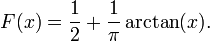
Density function:

$f(x) = \frac{1}{{\pi}(1+x^2)}.$

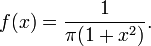
See Cauchy distribution

ν = 2

Distribution function:

$F(x) = \frac{1}{2}\left[1+\frac{x}{\sqrt{2+x^2}}\right].$

Density function:

$f(x) = \frac{1}{\left(2+x^2\right)^{3/2}}.$

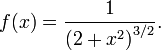
Robust parametric modelling

The t-distribution is often used as an alternative to the normal distribution as a model for data. It is frequently the case that real data have heavier tails than the normal distribution allows for. The classical approach was to identify outliers and exclude or downweight them in some way. However, it is not always easy to identify outliers (especially in high dimensions), and the t-distribution is a natural choice of model for such data and provides a parametric approach to robust statistics.

Lange et al explored the use of the t-distribution for robust modelling of heavy tailed data in a variety of contexts. A Bayesian account can be found in Gelman et al. The degrees of freedom parameter controls the kurtosis of the distribution and is correlated with the scale parameter. The likelihood can have multiple local maxima and, as such, it is often necessary to fix the degrees of freedom at a fairly low value and estimate the other parameters taking this as given. Some authors report that values between 3 and 9 are often good choices. Venables and Ripley suggest that a value of 5 is often a good choice.

Related distributions

$X \sim \mathrm{t}(\nu)$ has a t-distribution if $\sigma^2 \sim \mbox{Inv-}\chi^2(\nu,1)\!$ has a scaled inverse-χ² distribution and $X \sim \mathrm{N}(0,\sigma^2)\!$ has a normal distribution.
$Y \sim \mathrm{F}(\nu_1 = 1, \nu_2 = \nu)$ has an F-distribution if $Y = X^2\!$ and $X \sim \mathrm{t}(\nu)\!$ has a Student's t-distribution.
$Y \sim \mathrm{N}(0,1)\!$ has a normal distribution as $Y = \lim_{\nu \to \infty} X$ where $X \sim \mathrm{t}(\nu)$ .
$X \sim \mathrm{Cauchy}(0,1)$ has a Cauchy distribution if $X \sim \mathrm{t}(\nu = 1)$ .