Variance

Related subjects: Mathematics

Background Information

SOS Children produced this website for schools as well as this video website about Africa. SOS Children has looked after children in Africa for forty years. Can you help their work in Africa?

In probability theory and statistics, the variance of a random variable, probability distribution, or sample is one measure of statistical dispersion, averaging the squared distance of its possible values from the expected value (mean). Whereas the mean is a way to describe the location of a distribution, the variance is a way to capture its scale or degree of being spread out. The unit of variance is the square of the unit of the original variable. The square root of the variance, called the standard deviation, has the same units as the original variable and can be easier to interpret for this reason.

The variance of a real-valued random variable is its second central moment, and it also happens to be its second cumulant. Just as some distributions do not have a mean, some do not have a variance as well. The mean exists whenever the variance exists, but not vice versa.

Definition

If μ = E(X) is the expected value (mean) of the random variable X, then the variance is

$\operatorname{Var}(X) = \operatorname{E}[ ( X - \mu ) ^ 2 ].\,$

This definition encompasses random variables that are discrete, continuous, or neither. Of all the points about which squared deviations could have been calculated, the mean produces the minimum value for the averaged sum of squared deviations.

Many distributions, such as the Cauchy distribution, do not have a variance because the relevant integral diverges. In particular, if a distribution does not have an expected value, it does not have a variance either. The converse is not true: there are distributions for which the expected value exists, but the variance does not.

Discrete case

If the random variable is discrete with probability mass function p₁, ..., p_n, this is equivalent to

$\sum_{i=1}^n (x_i - \mu)^2 p_i\,.$

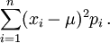
(Note: this variance should be divided by the sum of weights in the case of a discrete weighted variance.) That is, it is the expected value of the square of the deviation of X from its own mean. In plain language, it can be expressed as "The average of the square of the distance of each data point from the mean". It is thus the mean squared deviation. The variance of random variable X is typically designated as Var(X), $\scriptstyle\sigma_X^2$ , or simply σ².

Properties

Variance is non-negative because the squares are positive or zero. The variance of a random variable is 0 if and only if the variable is degenerate, that is, it takes on a constant value with probability 1, and the variance of a variable in a data set is 0 if and only if all entries have the same value.

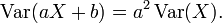
Variance is invariant with respect to changes in a location parameter. That is, if a constant is added to all values of the variable, the variance is unchanged. If all values are scaled by a constant, the variance is scaled by the square of that constant. These two properties can be expressed in the following formula:

$\operatorname{Var}(aX+b)=a^2\operatorname{Var}(X).$

The variance of a finite sum of uncorrelated random variables is equal to the sum of their variances.

Suppose that the observations can be partitioned into subgroups according to some second variable. Then the variance of the total group is equal to the mean of the variances of the subgroups plus the variance of the means of the subgroups. This property is known as variance decomposition or the law of total variance and plays an important role in the analysis of variance. For example, suppose that a group consists of a subgroup of men and an equally large subgroup of women. Suppose that the men have a mean body length of 180 and that the variance of their lengths is 100. Suppose that the women have a mean length of 160 and that the variance of their lengths is 50. Then the mean of the variances is (100 + 50) / 2 = 75; the variance of the means is the variance of 180, 160 which is 100. Then, for the total group of men and women combined, the variance of the body lengths will be 75 + 100 = 175. Note that this uses N for the denominator instead of N - 1.
In a more general case, if the subgroups have unequal sizes, then they must be weighted proportionally to their size in the computations of the means and variances. The formula is also valid with more than two groups, and even if the grouping variable is continuous.

This formula implies that the variance of the total group cannot be smaller than the mean of the variances of the subgroups. Note, however, that the total variance is not necessarily larger than the variances of the subgroups. In the above example, when the subgroups are analyzed separately, the variance is influenced only by the man-man differences and the woman-woman differences. If the two groups are combined, however, then the men-women differences enter into the variance also.
Many computational formulas for the variance are based on this equality: The variance is equal to the mean of the squares minus the square of the mean. For example, if we consider the numbers 1, 2, 3, 4 then the mean of the squares is (1 × 1 + 2 × 2 + 3 × 3 + 4 × 4) / 4 = 7.5. The mean is 2.5, so the square of the mean is 6.25. Therefore the variance is 7.5 − 6.25 = 1.25, which is indeed the same result obtained earlier with the definition formulas. Many pocket calculators use an algorithm that is based on this formula and that allows them to compute the variance while the data are entered, without storing all values in memory. The algorithm is to adjust only three variables when a new data value is entered: The number of data entered so far (n), the sum of the values so far (S), and the sum of the squared values so far (SS). For example, if the data are 1, 2, 3, 4, then after entering the first value, the algorithm would have n = 1, S = 1 and SS = 1. After entering the second value (2), it would have n = 2, S = 3 and SS = 5. When all data are entered, it would have n = 4, S = 10 and SS = 30. Next, the mean is computed as M = S / n, and finally the variance is computed as SS / n − M × M. In this example the outcome would be 30 / 4 - 2.5 × 2.5 = 7.5 − 6.25 = 1.25. If the unbiased sample estimate is to be computed, the outcome will be multiplied by n / (n − 1), which yields 1.667 in this example.

Properties, formal

8.a. Variance of the sum of uncorrelated variables

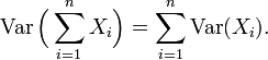
One reason for the use of the variance in preference to other measures of dispersion is that the variance of the sum (or the difference) of uncorrelated random variables is the sum of their variances:

$\operatorname{Var}\Big(\sum_{i=1}^n X_i\Big) = \sum_{i=1}^n \operatorname{Var}(X_i).$

This statement is often made with the stronger condition that the variables are independent, but uncorrelatedness suffices. So if the variables have the same variance σ², then, since division by n is a linear transformation, this formula immediately implies that the variance of their mean is

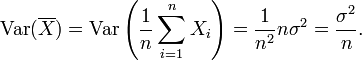
$\operatorname{Var}(\overline{X}) = \operatorname{Var}\left(\frac{1}{n}\sum_{i=1}^n X_i\right) = \frac {1}{n^2} n \sigma^2 = \frac {\sigma^2} {n}.$

That is, the variance of the mean decreases with n. This fact is used in the definition of the standard error of the sample mean, which is used in the central limit theorem.

8.b. Variance of the sum of correlated variables

In general, if the variables are correlated, then the variance of their sum is the sum of their covariances:

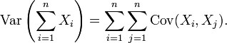
$\operatorname{Var}\left(\sum_{i=1}^n X_i\right) = \sum_{i=1}^n \sum_{j=1}^n \operatorname{Cov}(X_i, X_j).$

Here Cov is the covariance, which is zero for independent random variables (if it exists). The formula states that the variance of a sum is equal to the sum of all elements in the covariance matrix of the components. This formula is used in the theory of Cronbach's alpha in classical test theory.

So if the variables have equal variance σ² and the average correlation of distinct variables is ρ, then the variance of their mean is

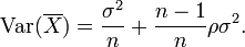
$\operatorname{Var}(\overline{X}) = \frac {\sigma^2} {n} + \frac {n-1} {n} \rho \sigma^2.$

This implies that the variance of the mean increases with the average of the correlations. Moreover, if the variables have unit variance, for example if they are standardized, then this simplifies to

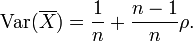
$\operatorname{Var}(\overline{X}) = \frac {1} {n} + \frac {n-1} {n} \rho.$

This formula is used in the Spearman-Brown prediction formula of classical test theory. This converges to ρ if n goes to infinity, provided that the average correlation remains constant or converges too. So for the variance of the mean of standardized variables with equal correlations or converging average correlation we have

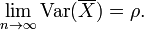
$\lim_{n \to \infty} \operatorname{Var}(\overline{X}) = \rho.$

Therefore, the variance of the mean of a large number of standardized variables is approximately equal to their average correlation. This makes clear that the sample mean of correlated variables does generally not converge to the population mean, even though the Law of large numbers states that the sample mean will converge for independent variables.

8.c. Variance of a weighted sum of variables

Properties 6 and 8, along with this property from the covariance page: Cov(aX, bY) = ab Cov(X, Y) jointly imply that

$\operatorname{Var}(aX+bY) =a^2 \operatorname{Var}(X) + b^2 \operatorname{Var}(Y) + 2ab\, \operatorname{Cov}(X, Y).$

This implies that in a weighted sum of variables, the variable with the largest weight will have a disproportionally large weight in the variance of the total. For example, if X and Y are uncorrelated and the weight of X is two times the weight of Y, then the weight of the variance of X will be four times the weight of the variance of Y.

9. Decomposition of variance

The general formula for variance decomposition or the law of total variance is: If X and Y are two random variables and the variance of X exists, then

$\operatorname{Var}(X) = \operatorname{Var}(\operatorname{E}(X|Y))+ \operatorname{E}(\operatorname{Var}(X|Y)).$

Here, E(X|Y) is the conditional expectation of X given Y, and Var(X|Y) is the conditional variance of X given Y. (A more intuitive explanation is that given a particular value of Y, then X follows a distribution with mean E(X|Y) and variance Var(X|Y). The above formula tells how to find Var(X) based on the distributions of these two quantities when Y is allowed to vary.) This formula is often applied in analysis of variance, where the corresponding formula is

$SS_{\mbox{Total}} = SS_{\mbox{Between}} + SS_{\mbox{Within}}.$

It is also used in linear regression analysis, where the corresponding formula is

$SS_{\mbox{Total}} = SS_{\mbox{Regression}} + SS_{\mbox{Residual}}.$

This can also be derived from the additivity of variances (property 8), since the total (observed) score is the sum of the predicted score and the error score, where the latter two are uncorrelated.

10. Computational formula for variance

The computational formula for the variance follows in a straightforward manner from the linearity of expected values and the above definition:

${}\operatorname{Var}(X)= \operatorname{E}(X^2 - 2\,X\,\operatorname{E}(X) + (\operatorname{E}(X))^2),$

${}=\operatorname{E}(X^2) - 2(\operatorname{E}(X))^2 + (\operatorname{E}(X))^2,$

${}=\operatorname{E}(X^2) - (\operatorname{E}(X))^2.$

This is often used to calculate the variance in practice, although it suffers from numerical approximation error if the two components of the equation are similar in magnitude.

Characteristic property

The second moment of a random variable attains the minimum value when taken around the mean of the random variable, i.e. $\mathrm{E} X = \mathrm{argmin}_a \mathrm{E} (X - a)^2$ . This property could be reversed, i.e. if the function $\phi$ satisfies $\mathrm{E} X = \mathrm{argmin}_a \mathrm{E} \phi(X - a)$ then it is necessary of the form $\phi = a x^2 + b$ . This is also true in multidimensional case .

Approximating the variance of a function

The delta method uses second-order Taylor expansions to approximate the variance of a function of one or more random variables. For example, the approximate variance of a function of one variable is given by

$\operatorname{Var}\left[f(X)\right]\approx \left(f'(\operatorname{E}\left[X\right])\right)^2\operatorname{Var}\left[X\right]$

provided that f is twice differentiable and that the mean and variance of X are finite.

Generalizations

If $X$ is a vector-valued random variable, with values in $\mathbb{R}^n$ , and thought of as a column vector, then the natural generalization of variance is $\operatorname{E}((X - \mu)(X - \mu)^\operatorname{T})$ , where $\mu = \operatorname{E}(X)$ and $X^\operatorname{T}$ is the transpose of $X$ , and so is a row vector. This variance is a positive semi-definite square matrix, commonly referred to as the covariance matrix.

If $X$ is a complex-valued random variable, with values in $\mathbb{C}$ , then its variance is $\operatorname{E}((X - \mu)(X - \mu)^*)$ , where $X^*$ is the complex conjugate of $X$ . This variance is also a positive semi-definite square matrix.

History

The term variance was first introduced by Ronald Fisher in his 1918 paper The Correlation Between Relatives on the Supposition of Mendelian Inheritance.

Moment of inertia

The variance of a probability distribution is analogous to the moment of inertia in classical mechanics of a corresponding mass distribution along a line, with respect to rotation about its centre of mass. It is because of this analogy that such things as the variance are called moments of probability distributions. (The covariance matrix is analogous to the moment of inertia tensor for multivariate distributions.)

Retrieved from " http://en.wikipedia.org/w/index.php?title=Variance&oldid=195568864"

We provide Linux to the World