

Quantum computer
Did you know...
The articles in this Schools selection have been arranged by curriculum topic thanks to SOS Children volunteers. Before you decide about sponsoring a child, why not learn about different sponsorship charities first?

A quantum computer is a device for computation that makes direct use of distinctively quantum mechanical phenomena, such as superposition and entanglement, to perform operations on data. In a classical (or conventional) computer, information is stored as bits; in a quantum computer, it is stored as qubits (quantum binary digits). The basic principle of quantum computation is that the quantum properties can be used to represent and structure data, and that quantum mechanisms can be devised and built to perform operations with this data.
Although quantum computing is still in its infancy, experiments have been carried out in which quantum computational operations were executed on a very small number of qubits. Both practical and theoretical research continues with interest, and many national government and military funding agencies support quantum computing research to develop quantum computers for both civilian and national security purposes, such as cryptanalysis.
If large-scale quantum computers can be built, they will be able to solve certain problems much faster than any of our current classical computers (for example Shor's algorithm). Quantum computers are different from other computers such as DNA computers and traditional computers based on transistors. Some computing architectures such as optical computers may use classical superposition of electromagnetic waves. Without some specifically quantum mechanical resources such as entanglement, it is conjectured that an exponential advantage over classical computers is not possible.
Basis
A classical computer has a memory made up of bits, where each bit holds either a one or a zero. A quantum computer maintains a sequence of qubits. A single qubit can hold a one, a zero, or, crucially, a quantum superposition of these; moreover, a pair of qubits can be in a quantum superposition of 4 states, and three qubits in a superposition of 8. In general a quantum computer with n qubits can be in up to  different states simultaneously (this compares to a normal computer that can only be in one of these states at any one time). A quantum computer operates by manipulating those qubits with a fixed sequence of quantum logic gates. The sequence of gates to be applied is called a quantum algorithm.
An example of an implementation of qubits for a quantum computer could start with the use of particles with two spin states: "up" and "down" (typically written  and
and  , or
, or  and
and  ). But in fact any system possessing an observable quantity A which is conserved under time evolution and such that A has at least two discrete and sufficiently spaced consecutive eigenvalues, is a suitable candidate for implementing a qubit. This is true because any such system can be mapped onto an effective spin-1/2 system.
Bits vs. Qubits

Consider first a classical computer that operates on a three-bit register. The state of the computer at any time is a probability distribution over the  different three-bit strings 000, 001, ..., 111—thus it is described by eight nonnegative numbers (a,b,c,d,e,f,g,h)—adding up to one.
The state of a three-qubit quantum computer is similarly described by an eight-dimensional vector (a,b,c,d,e,f,g,h), called a wavefunction. However, instead of adding to one, the sum of the squares of the coefficient magnitudes,  , must equal one. Moreover, the coefficients are complex numbers that need not be nonnegative. The fact that the coefficients can be negative as well as positive allows for cancellation, or interference, between different computational paths, and is a key difference between quantum computing and probabilistic classical computing.
If you measure the three qubits, then you will observe a three-bit string. The probability of measuring a string will equal the squared magnitude of that string's coefficients. Thus a measurement of the quantum state with coefficients (a,b,...,h) gives the classical probability distribution  . We say that the quantum state "collapses" to a classical state.
Note that an eight-dimensional vector can be specified in many different ways, depending on what basis you choose for the space. The basis of three-bit strings 000, 001, ..., 111 is known as the computational basis, and is often convenient, but other bases of unit-length, orthogonal vectors can also be used. Ket notation is often used to make explicit the choice of basis. For example, the state (a,b,c,d,e,f,g,h) in the computational basis can be written as  , where, e.g.,
  = (0,0,1,0,0,0,0,0). The computational basis for a single qubit (two dimensions) is = (1,0), = (0,1), but another common basis is the Hadamard basis of
  and
and 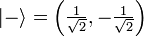 .
.
Note that although recording a classical state of n bits, a 2n-dimensional probability distribution, requires an exponential number of real numbers, practically we can always think of the system as being exactly one of the n-bit strings—we just don't know which one. Quantumly, this is no longer the case, and all 2n complex coefficients need to be kept track of to see how the quantum system evolves. For example, a 300-qubit quantum computer has a state described by 2300 (approximately 1090) complex numbers, more than the number of atoms in the observable universe.
Operation
While a classical three-bit state and a quantum three-qubit state are both eight-dimensional vectors, they are manipulated quite differently for classical or quantum computation, respectively. For computing in either case, the system must be initialized, for example into the all-zeros string, i.e., (1,0,0,0,0,0,0,0) or  . In classical randomized computation, the system evolves according to the application of stochastic matrices, which preserve that the probabilities add up to one (i.e., preserve the L1 norm). In quantum computation, on the other hand, allowed operations are unitary matrices, which are effectively rotations (they preserve that the sum of the squares add up to one, the Euclidean or L2 norm). (Exactly what unitaries can be applied depend on the physics of the quantum device.) Consequently, since rotations can be undone by rotating backward, quantum computations are reversible. (Technically, quantum operations can be probabilistic combinations of unitaries, so quantum computation really does generalize classical computation. See quantum circuit for a more precise formulation.)
Finally, upon termination of the algorithm, the result needs to be read off. In the case of a classical computer, we sample from the probability distribution on the three-bit register to obtain one definite three-bit string, say 000. Quantumly, we measure the three-qubit state, which is equivalent to collapsing the quantum state down to a classical distribution (with the coefficients in the classical state being the squared magnitudes of the coefficients for the quantum state, as described above) followed by sampling from that distribution. Note that this destroys the original quantum state. Many algorithms will only give the correct answer with a certain probability, however by repeatedly initializing, running and measuring the quantum computer, the probability of getting the correct answer can be increased. For example, running the Shor factorisation algorithm four times will give the correct answer with a very high probability.
For more details on the sequences of operations used for various algorithms, see universal quantum computer, Shor's algorithm, Grover's algorithm, Deutsch-Jozsa algorithm, quantum Fourier transform, quantum gate, quantum adiabatic algorithm and quantum error correction.
Potential
Integer factorization is believed to be computationally infeasible with an ordinary computer for large integers that are the product of only a few prime numbers (e.g., products of two 300-digit primes). By comparison, a quantum computer could efficiently solve this problem using Shor's algorithm to find its factors. This ability would allow a quantum computer to "break" many of the cryptographic systems in use today, in the sense that there would be a polynomial time (in the number of bits of the integer) algorithm for solving the problem. In particular, most of the popular public key ciphers are based on the difficulty of factoring integers (or the related discrete logarithm problem which can also be solved by Shor's algorithm), including forms of RSA. These are used to protect secure Web pages, encrypted email, and many other types of data. Breaking these would have significant ramifications for electronic privacy and security. The only way to increase the security of an algorithm like RSA would be to increase the key size and hope that an adversary does not have the resources to build and use a powerful enough quantum computer.
A way out of this dilemma would be to use some kind of quantum cryptography. There are also some digital signature schemes that are believed to be secure against quantum computers. See for instance Lamport signatures.
This dramatic advantage of quantum computers has only been discovered for factorization and discrete logarithms so far. However, there is no proof that the advantage is real: an equally fast classical algorithm may still be discovered. There is one other problem where quantum computers have a smaller, though significant (quadratic) advantage. It is quantum database search, and can be solved by Grover's algorithm. In this case the advantage is provable. This establishes beyond doubt that (ideal) quantum computers are superior to classical computers for at least one problem.
Consider a problem that has these four properties:
- The only way to solve it is to guess answers repeatedly and check them,
- There are n possible answers to check,
- Every possible answer takes the same amount of time to check, and
- There are no clues about which answers might be better: generating possibilities randomly is just as good as checking them in some special order.
An example of this is a password cracker that attempts to guess the password for an encrypted file (assuming that the password has a maximum possible length).
For problems with all four properties, the time for a quantum computer to solve this will be proportional to the square root of n (it would take an average of (n + 1)/2 guesses to find the answer using a classical computer.) That can be a very large speedup, reducing some problems from years to seconds. It can be used to attack symmetric ciphers such as Triple DES and AES by attempting to guess the secret key. Regardless of whether any of these problems can be shown to have an advantage on a quantum computer, they nonetheless will always have the advantage of being an excellent tool for studying quantum mechanical interactions, which of itself is an enormous value to the scientific community.
Grover's algorithm can also be used to obtain a quadratic speed-up [over a brute-force search] for a class of problems known as NP-complete.
Problems
There are a number of practical difficulties in building a quantum computer, and thus far quantum computers have only solved trivial problems. David DiVincenzo, of IBM, listed the following requirements for a practical quantum computer:
- scalable physically to increase the number of qubits
- qubits can be initialized to arbitrary values
- quantum gates faster than decoherence time
- universal gate set
- qubits can be read easily
To summarize the problems from the perspective of an engineer, one needs to solve the challenge of building a system which is isolated from everything except the measurement and manipulation mechanism. Furthermore, one needs to be able to turn off the coupling of the qubits to the measurement so as to not decohere the qubits while performing operations on them.
Quantum decoherence
One major problem is keeping the components of the computer in a coherent state, as the slightest interaction with the external world would cause the system to decohere. This effect causes the unitary character (and more specifically, the invertibility) of quantum computational steps to be violated. Decoherence times for candidate systems, in particular the transverse relaxation time T2 (terminology used in NMR and MRI technology, also called the dephasing time), typically range between nanoseconds and seconds at low temperature. The issue for optical approaches are more difficult as these timescales are orders of magnitude lower and an often cited approach to overcome it uses an optical pulse shaping approach. Error rates are typically proportional to the ratio of operating time to decoherence time, hence any operation must be completed much more quickly than the decoherence time.
If the error rate is small enough, it is thought to be possible to use quantum error correction, which corrects errors due to decoherence, thereby allowing the total calculation time to be longer than the decoherence time. An often cited (but rather arbitrary) figure for required error rate in each gate is 10−4. This implies that each gate must be able to perform its task 10,000 times faster than the decoherence time of the system.
Meeting this scalability condition is possible for a wide range of systems. However, the use of error correction brings with it the cost of a greatly increased number of required qubits. The number required to factor integers using Shor's algorithm is still polynomial, and thought to be between L and L2, where L is the number of bits in the number to be factored; error correction algorithms would inflate this figure by an additional factor of L. For a 1000-bit number, this implies a need about 104 qubits without error correction. With error correction, the figure would rise to about 107 qubits. Note that computation time is about  or about
  steps and on 1 M Hz, about 10 seconds.
A very different approach to the stability-decoherence problem is to create a topological quantum computer with anyons, quasi-particles used as threads and relying on braid theory to form stable logic gates.
Candidates
There are a number of quantum computing candidates, among those:
- Superconductor-based quantum computers (including SQUID-based quantum computers)
- Trapped ion quantum computer
- Optical lattices
- Topological quantum computer
- Quantum dot on surface (e.g. the Loss-DiVincenzo quantum computer)
- Nuclear magnetic resonance on molecules in solution (liquid NMR)
- Solid state NMR Kane quantum computers
- Electrons on helium quantum computers
- Cavity quantum electrodynamics (CQED)
- Molecular magnet
- Fullerene-based ESR quantum computer
- Optic-based quantum computers ( Quantum optics)
- Diamond-based quantum computer
- Bose–Einstein condensate-based quantum computer
- Transistor-based quantum computer - string quantum computers with entrainment of positive holes using a electrostatic trap
- Spin-based quantum computer
- Adiabatic quantum computation
The large number of candidates shows explicitly that the topic, in spite of rapid progress, is still in its infancy. But at the same time there is also a vast amount of flexibility.
In 2005, researchers at the University of Michigan built a semiconductor chip which functioned as an ion trap. Such devices, produced by standard lithography techniques, may point the way to scalable quantum computing tools. An improved version was made in 2006.
Quantum computing in computational complexity theory

This section surveys what is currently known mathematically about the power of quantum computers. It describes the known results from computational complexity theory and the theory of computation dealing with quantum computers.
The class of problems that can be efficiently solved by quantum computers is called BQP, for "bounded error, quantum, polynomial time". Quantum computers only run probabilistic algorithms, so BQP on quantum computers is the counterpart of BPP on classical computers. It is defined as the set of problems solvable with a polynomial-time algorithm, whose probability of error is bounded away from one quarter. A quantum computer is said to "solve" a problem if, for every instance, its answer will be right with high probability. If that solution runs in polynomial time, then that problem is in BQP.
BQP is contained in the complexity class #P (or more precisely in the associated class of decision problems P#P) , which is a subclass of PSPACE.
BQP is suspected to be disjoint from NP-complete and a strict superset of P, but that is not known. Both integer factorization and discrete log are in BQP. Both of these problems are NP problems suspected to be outside BPP, and hence outside P. Both are suspected to not be NP-complete. There is a common misconception that quantum computers can solve NP-complete problems in polynomial time. That is not known to be true, and is generally suspected to be false.
Quantum gates may be viewed as linear transformations. Daniel S. Abrams and Seth Lloyd have shown that if nonlinear transformations are permitted, then NP-complete problems could be solved in polynomial time. It could even do so for #P-complete problems. They do not believe that such a machine is possible.
Although quantum computers may be faster than classical computers, those described above can't solve any problems that classical computers can't solve, given enough time and memory (albeit possibly an amount that could never practically be brought to bear). A Turing machine can simulate these quantum computers, so such a quantum computer could never solve an undecidable problem like the halting problem. The existence of "standard" quantum computers does not disprove the Church-Turing thesis.