

First-order logic
Background to the schools Wikipedia
This Schools selection was originally chosen by SOS Children for schools in the developing world without internet access. It is available as a intranet download. A quick link for child sponsorship is http://www.sponsor-a-child.org.uk/
First-order logic (FOL) is a formal deductive system used by mathematicians, philosophers, linguists, and computer scientists. It goes by many names, including: first-order predicate calculus (FOPC), the lower predicate calculus, the language of first-order logic or predicate logic. Unlike natural languages such as English, FOL uses a wholly unambiguous formal language interpreted by mathematical structures. FOL is a system of deduction extending propositional logic by allowing quantification over individuals of a given domain (universe) of discourse. For example, it can be stated in FOL "Every individual has the property P".
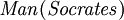
While propositional logic deals with simple declarative propositions, first-order logic additionally covers predicates and quantification. Take for example the following sentences: "Socrates is a man", "Plato is a man". In propositional logic these will be two unrelated propositions, denoted for example by p and q. In first-order logic however, both sentences would be connected by the same property: Man(x), where Man(x) means that x is a man. When x=Socrates we get the first proposition, p, and when x=Plato we get the second proposition, q. Such a construction allows for a much more powerful logic when quantifiers are introduced, such as "for every x...", for example, "for every x, if Man(x), then...". Without quantifiers, every valid argument in FOL is valid in propositional logic, and vice versa.
A first-order theory consists of a set of axioms (usually finite or recursively enumerable) and the statements deducible from them given the underlying deducibility relation. Usually what is meant by 'first-order theory' is some set of axioms together with those of a complete (and sound) axiomatization of first-order logic, closed under the rules of FOL. (Any such system FOL will give rise to the same abstract deducibility relation, so we needn't have a fixed axiomatic system in mind.) A first-order language has sufficient expressive power to formalize two important mathematical theories: ZFC set theory and Peano arithmetic. A first-order language cannot, however, categorically express the notion of countability even though it is expressible in the first-order theory ZFC under the intended interpretation of the symbolism of ZFC. Such ideas can be expressed categorically with second-order logic.
Why is first-order logic needed?
Propositional logic is not adequate for formalizing valid arguments that rely on the internal structure of the propositions involved. To see this, consider the valid syllogistic argument:
- All men are mortal
- Socrates is a man
- Therefore, Socrates is mortal
which upon translation into propositional logic yields:
- A
- B
 C
C
(taking to mean "therefore").
According to propositional logic, this translation is invalid: Propositional logic validates arguments according to their structure, and nothing in the structure of this translated argument (C follows from A and B, for arbitrary A, B, C) suggests that it is valid. A translation that preserves the intuitive (and formal) validity of the argument must take into consideration the deeper structure of propositions, such as the essential notions of predication and quantification. Propositional logic deals only with truth-functional validity: any assignment of truth-values to the variables of the argument should make either the conclusion true or at least one of the premises false. Clearly we may (uniformly) assign truth values to the variables of the above argument such that A, B are both true but C is false. Hence the argument is truth-functionally invalid. On the other hand, it is impossible to (uniformly) assign truth values to the argument "A follows from (A and B)" such that (A and B) is true (hence A is true and B is true) and A false.
In contrast, this argument can be easily translated into first-order logic:

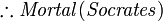
(Where " " means "for all x", "
 " means "implies",
 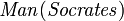 means "Socrates is a man", and
  means "Socrates is mortal".) In plain English, this states that
- for all x, if x is a man then x is mortal
- Socrates is a man
- therefore Socrates is mortal
FOL can also express the existence of something ( ), as well as predicates ("functions" that are true or false) with more than one parameter. For example, "there is someone who can be fooled every time" can be expressed as:

Where " " means "there exists (an) x", "
 " means "and", and
 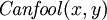 means "(person) x can be fooled (at time) y".
Defining first-order logic
A predicate calculus consists of
- formation rules (i.e. recursive definitions for forming well-formed formulas).
- transformation rules (i.e. inference rules for deriving theorems).
- axioms or axiom schemata (possibly countably infinite).
The axioms considered here are logical axioms which are part of classical FOL. It is important to note that FOL can be formalized in many equivalent ways; there is nothing canonical about the axioms and rules of inference given in this article. There are infinitely many equivalent formalizations all of which yield the same theorems and non-theorems, and all of which have equal right to the title 'FOL'.
FOL is used as the basic "building block" for many mathematical theories. FOL provides several built-in rules, such as the axiom 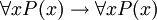 (if P(x) is true for every x then P(x) is true for every x). Additional non-logical axioms are added to produce specific first-order theories based on the axioms of classical FOL; these theories built on FOL are called classical first-order theories. One example of a classical first-order theory is Peano arithmetic, which adds to axiom
 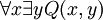 (i.e. for every x there exists y such that y=x+1, where Q(x,y) is interpreted as "y=x+1"). This additional axiom is a non-logical axiom; it is not part of FOL, but instead is an axiom of the theory (an axiom of arithmetic rather than of logic). Axioms of the latter kind are also called axioms of first-order theories. The axioms of first-order theories are not regarded as truths of logic per se, but rather as truths of the particular theory that usually has associated with it an intended interpretation of its non-logical symbols. (See an analogous idea at logical versus non-logical symbols.) Thus, the axiom about Q(x,y) is true only with the interpretation of the relation Q(x,y) as "y=x+1", and only in the theory of Peano arithmetic. Classical FOL does not have associated with it an intended interpretation of its non-logical vocabulary (except arguably a symbol denoting identity, depending on whether one regards such a symbol as logical). Classical set-theory is another example of a first-order theory (a theory built on FOL).
Vocabulary
Before setting up the formation rules, one has to describe the "vocabulary", which is composed of
- A set of predicate variables (or relations) each with some valence (or arity, number of its arguments) ≥1, which are often denoted by uppercase letters P, Q, R,... .
- For example, P(x) is a predicate variables of valence 1. It can stand for "x is a man", for example.
- Q(x,y) is a predicate variables of valence 2. It can stand for "x is greater than y" in arithmetic or "x is the father of y", for example.
- It is possible to allow relations of valence 0; these could be considered as propositional variables. For example, P, which can stand for any statement.
- By using functions (see below), it is possible to dispense with all predicate variables with valence larger than one. For example, "x>y" (a predicate of valence 2, of the type Q(x,y)) can be replaced by a predicate of valence 1 about the ordered pair (x,y).
- A set of constants, often denoted by lowercase letters at the beginning of the alphabet a, b, c,... .
- Examples: a may stand for Socrates. In arithmetic, it may stand for 0. In set theory, such a constant may stand for the empty set.
- A set of functions, each of some valence ≥ 1, which are often denoted by lowercase letters f, g, h,... .
- Examples: f(x) may stand for "the father of x". In arithmetic, it may stand for "-x". In set theory, it may stand for "the power set of x". In arithmetic, f(x,y) may stand for "x+y". In set theory, it may stand for "the union of x and y".
- A constant is really a function of valence 0. However it is traditional to use the term "function" only for functions of valence at least 1.
- One can in principle dispense entirely with functions of arity > 2 and predicates of arity > 1 if there is a function symbol of arity 2 representing an ordered pair (or predicate symbols of arity 2 representing the projection relations of an ordered pair). The pair or projections need to satisfy the natural axioms.
- One can in principle dispense entirely with functions and constants. For example, instead of using a constant 0 one may use a predicate 0(x) (interpreted as "x=0"), and replace every predicate such as P(0,y) with
 x 0(x) P(x,y). A function such as f(x1,x2...) will similarly be replaced by a predicate F(x1,x2...,y) (interpreted as "y=f(x1,x2...)").
- An infinite set of variables, often denoted by lowercase letters at the end of the alphabet x, y, z,... .
- Symbols denoting logical operators (or connectives):
 ( logical not), ( logical conditional).
 - (φ ψ) is logically equivalent to φ
 ψ ( logical and). φ ψ can be seen as a shorthand for this. Alternatively, one may add the symbol as a logical operator to the vocabulary, and appropriate axioms.
 - φ ψ is logically equivalent to φ
 ψ ( logical or). φ ψ can be seen as a shorthand for this. Alternatively, one may add the symbol as a logical operator to the vocabulary, and appropriate axioms.
 - Similarly, (φψ)(ψφ) is logically equivalent to φ
 ψ ( logical biconditional), and one may use the latter as a shorthand for this, or alternatively add this to the vocabulary and add appropriate axioms. Sometimes φ ψ is written as φ
  ψ.
ψ.
- Symbols denoting quantifiers: ( universal quantification, typically read as "for all").
 xφ) is logically equivalent to x φ ( existential quantification, typically read as "there exists"). The latter can either be used as a shorthand for this, or added to the vocabulary together with appropriate axioms.
- Left and right parenthesis.
- There are many different conventions about where to put parentheses; for example, one might write x or (x). Sometimes one uses colons or full stops instead of parentheses to make formulas unambiguous. One interesting but rather unusual convention is " Polish notation", where one omits all parentheses, and writes , , and so on in front of their arguments rather than between them. Polish notation is compact and elegant, but rare because it is hard for humans to read it.
- There are many different conventions about where to put parentheses; for example, one might write
- An identity or equality symbol = is sometimes but not always included in the vocabulary.
- If equality is considered to be a part of first-order logic, then the equality symbol behaves syntactically as a binary predicate. This case is sometimes called first-order logic with equality.
There are several further minor variations listed below:
- The set of primitive symbols (operators and quantifiers) often varies. It is possible to include other operators as primitive, such as (iff), (and) and (or), the truth constants T for "true" and F for "false" (these are operators of valence 0), and/or the Sheffer stroke (P | Q, aka NAND). The minimum number of primitive symbols needed is one, but if we restrict ourselves to the operators listed above, we need three, as above.
- Some books and papers use the notation φ
 ψ for φ ψ. This is especially common in proof theory where is easily confused with the sequent arrow. One also sees ~φ for φ, φ & ψ for φ ψ, and a wealth of notations for quantifiers; e.g., x φ may be written as (x)φ. This latter notation is common in texts on recursion theory.
 - It is often easier in practice to use a simpler notation that supports infix operators and omits unnecessary parentheses. Thus if P is a relation of valence 2, we often write "a P b" instead of "P a b"; for example, we write 1 < 2 instead of <(1 2). Similarly if f is a function of valence 2, we sometimes write "a f b" instead of "f(a b)"; for example, we write 1 + 2 instead of +(1 2). By convention, infix operators tend to use non-alphabetic function names. It is also common to omit some parentheses if this does not lead to ambiguity (leading to defining a precedence).
- Sometimes it is useful to say that "P(x) holds for exactly one x", which can be expressed as
 x P(x). This notation may be taken to abbreviate a formula such as x (P(x)
  y (P(y) (x = y))) .
Computer programs that accept first-order logic representations will typically accept at least these quantifiers and operators (though they may use different symbols to represent them): (forall), (exists), (not), (and), (or), (implies), and (if and only if). The exclusive-or operator "xor" is also common.
The sets of constants, functions, and relations are usually considered to form a language, while the variables, logical operators, and quantifiers are usually considered to belong to the logic. For example, the language of group theory consists of one constant (the identity element), one function of valence 1 (the inverse) one function of valence 2 (the product), and one relation of valence 2 (equality), which would be omitted by authors who include equality in the underlying logic.
Formation rules
The formation rules define the terms and formulas of first order logic. When terms and formulas are represented as strings of symbols, these rules can be used to write a formal grammar for terms and formulas. The concept of free variable is used to define the sentences as a subset of the formulas.
Terms
The set of terms is recursively defined by the following rules:
- Any constant is a term.
- Any variable is a term.
- Any expression f(t1,...,tn) of n ≥ 1 arguments (where each argument ti is a term and f is a function symbol of valence n) is a term.
- Closure clause: Nothing else is a term. For example, predicates are not terms.
Formulas
The set of well-formed formulas (usually called wffs or just formulas) is recursively defined by the following rules:
- Simple and complex predicates If P is a relation of valence n ≥ 1 and the ai are terms then P(a1,...,an) is well-formed. If equality is considered part of logic, then (a1 = a2) is well formed. All such formulas are said to be atomic.
- Inductive Clause I: If φ is a wff, then φ is a wff.
- Inductive Clause II: If φ and ψ are wffs, then (φ ψ) is a wff.
- Inductive Clause III: If φ is a wff and x is a variable, then x φ is a wff.
- Closure Clause: Nothing else is a wff.
For example, x y (P(f(x))  (P(x) Q(f(y),x,z))) is a well-formed formula, if f is a function of valence 1, P a predicate of valence 1 and Q a predicate of valence 3. x x is not a well-formed formula.
In Computer science terminology, a formula implements a built-in "boolean" type, while a term implements all other types.
Free and Bound Variables
- Atomic formulas If φ is an Atomic formula then x is free in φ if and only if x occurs in φ.
- Inductive Clause I: x is free in φ if and only if x is free in φ.
- Inductive Clause II: x is free in (φ ψ) if and only if x is free in φ and does not occur in ψ, or x is free in ψ and does not occur in φ, or x is free in both φ and ψ.
- Inductive Clause III: x is free in y φ if and only if x is free in φ and x is a different symbol than y.
- Closure Clause: x is bound in φ if and only if x occurs in φ and x is not free in φ.
- For example, in x y (P(x) Q(x,f(x),z)), x and y are bound variables, z is a free variable, and w is neither because it does not occur in the formula.
Example
In mathematics the language of ordered abelian groups has one constant 0, one unary function −, one binary function +, and one binary relation ≤. So:
- 0, x, y are atomic terms
- +(x, y), +(x, +(y, −(z))) are terms, usually written as x + y, x + y − z
- =(+(x, y), 0), ≤(+(x, +(y, −(z))), +(x, y)) are atomic formulas, usually written as x + y = 0, x + y - z ≤ x + y,
- (x y ≤( +(x, y), z)) (x =(+(x, y), 0)) is a formula, usually written as (x y x + y ≤ z) (x x + y = 0).
Substitution
If t is a term and φ(x) is a formula possibly containing x as a free variable, then φ(t) is defined to be the result of replacing all free instances of x by t, provided that no free variable of t becomes bound in this process. If some free variable of t becomes bound, then to substitute t for x it is first necessary to change the names of bound variables of φ to something other than the free variables of t.
To see why this condition is necessary, consider the formula φ(x) given by y y ≤ x ("x is maximal"). If t is a term without y as a free variable, then φ(t) just means t is maximal. However if t is y the formula φ(y) is y y ≤ y which does not say that y is maximal. The problem is that the free variable y of t (=y) became bound when we substituted y for x in φ(x). So to form φ(y) we must first change the bound variable y of φ to something else, say z, so that φ(y) is then z z ≤ y. Forgetting this condition is a notorious cause of errors.
Inference rules
An inference rule is a function from sets of (well-formed) formulas, called premises, to sets of formulas called conclusions. In most well-known deductive systems, inference rules take a set of formulas to a single conclusion. (Notice this is true even in the case of most sequent calculi.)
Inference rules are used to prove theorems, which are formulas provable in or members of a theory. If the premises of an inference rule are theorems, then its conclusion is a theorem as well. In other words, inference rules are used to generate "new" theorems from "old" ones--they are theoremhood preserving. Systems for generating theories are often called predicate calculi. These are described in a section below.
An important inference rule, modus ponens, states that if φ and φ ψ are both theorems, then ψ is a theorem. This can be written as following;
- if
 and
and  , then
where indicates  is provable in theory T. There are deductive systems (known as Hilbert-style deductive systems) in which modus ponens is the sole rule of inference; in such systems, the lack of other inference rules is offset with an abundance of logical axiom schemes.
A second important inference rule is Universal Generalization. It can be stated as
- if , then

Which reads: if φ is a theorem, then "for every x, φ" is a theorem as well. The similar-looking schema  is not sound, in general, although it does however have valid instances, such as when x does not occur free in φ (see Generalization (logic)).
Axioms
Here follows a description of the axioms of first-order logic. As explained above, a given first-order theory has further, non-logical axioms. The following logical axioms characterize a predicate calculus for this article's example of first-order logic.
For any theory, it is of interest to know whether the set of axioms can be generated by an algorithm, or if there is an algorithm which determines whether a well-formed formula is an axiom.
If there is an algorithm to generate all axioms, then the set of axioms is said to be recursively enumerable.
If there is an algorithm which determines after a finite number of steps whether a formula is an axiom or not, then the set of axioms is said to be recursive or decidable. In that case, one may also construct an algorithm to generate all axioms: this algorithm simply builds all possible formulas one by one (with growing length), and for each formula the algorithm determines whether it is an axiom.
Axioms of first-order logic are always decidable. However, in a first-order theory non-logical axioms are not necessarily such.
Quantifier axioms
Quantifier axioms change according to how the vocabulary is defined, how the substitution procedure works, what are the formation rules and which inference rules are used. Here follows a specific example of these axioms
- PRED-1:
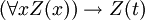
- PRED-2:
- PRED-3:

- PRED-4:

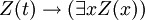
These are actually axiom schemata: the expression W stands for any wff in which x is not free, and the expression Z(x) stands for any wff with the additional convention that Z(t) stands for the result of substitution of the term t for x in Z(x). Thus this is a recursive set of axioms.
Another axiom,  , for Z in which x does not occur, is sometimes added.
Equality and its axioms
There are several different conventions for using equality (or identity) in first-order logic. This section summarizes the main ones. The various conventions all give essentially the same results with about the same amount of work, and differ mainly in terminology.
- The most common convention for equality is to include the equality symbol as a primitive logical symbol, and add the axioms for equality to the axioms for first-order logic. The equality axioms are
-
- x = x
- x = y → f(...,x,...) = f(...,y,...) for any function f
- x = y → (P(...,x,...) → P(...,y,...)) for any relation P (including the equality relation itself)
- These are, too, axiom schemata: they define an algorithm which decides whether a given formula is an axiom. Thus this is a recursive set of axioms.
- The next most common convention is to include the equality symbol as one of the relations of a theory, and add the equality axioms to the axioms of the theory. In practice this is almost indistinguishable from the previous convention, except in the unusual case of theories with no notion of equality. The axioms are the same, and the only difference is whether one calls some of them logical axioms or axioms of the theory.
- In theories with no functions and a finite number of relations, it is possible to define equality in terms of the relations, by defining the two terms s and t to be equal if any relation is unchanged by changing s to t in any argument.
-
- For example, in set theory with one relation
 , we may define s = t to be an abbreviation for x (s x t x) x (x s x t). This definition of equality then automatically satisfies the axioms for equality.
 - Alternatively, if one does use the equality symbol as a relation of the theory or of logic, then one would have to add axioms. In the previous example, one would have to add the axiom s t (x (x s x t)) s = t.
- For example, in set theory with one relation
- In some theories it is possible to give ad hoc definitions of equality. For example, in a theory of partial orders with one relation ≤ we could define s = t to be an abbreviation for s ≤ t t ≤ s.
Predicate calculus
The predicate calculus is a proper extension of the propositional calculus that defines which statements of first-order logic are provable. Many (but not all) mathematical theories can be formulated in the predicate calculus. If the propositional calculus is defined with a suitable set of axioms and the single rule of inference modus ponens (this can be done in many ways), then the predicate calculus can be defined by appending to the propositional calculus several axioms and the inference rule called "universal generalization". As axioms for the predicate calculus we take:
- All tautologies of the propositional calculus, taken schematically so that the uniform replacement of a schematic letter by a formula is allowed.
- The quantifier axioms, given above.
- The above axioms for equality, if equality is regarded as a logical concept.
A sentence is defined to be provable in first-order logic if it can be derived from the axioms of the predicate calculus, by repeatedly applying the inference rules "modus ponens" and "universal generalization". In other words:
- An axiom of the predicate calculus is provable in first-order logic by definition.
- If the premises of an inference rule are provable in first-order logic, then so is its conclusion.
If we have a theory T (a set of statements, called axioms, in some language) then a sentence φ is defined to be provable in the theory T if

is provable in first-order logic, for some finite set of axioms  of the theory T. In other words, if one can prove in first-order logic that φ follows from the axioms of T. This also means, that we replace the above procedure for finding provable sentences by the following one:
- An axiom of T is provable in T.
- An axiom of the predicate calculus is provable in T.
- If the premises of an inference rule are provable in T, then so is its conclusion.
One apparent problem with this definition of provability is that it seems rather ad hoc: we have taken some apparently random collection of axioms and rules of inference, and it is unclear that we have not accidentally missed out some vital axiom or rule. Gödel's completeness theorem assures us that this is not really a problem: any statement true in all models (semantically true) is provable in first-order logic (syntactically true). In particular, any reasonable definition of "provable" in first-order logic must be equivalent to the one above (though it is possible for the lengths of proofs to differ vastly for different definitions of provability).
There are many different (but equivalent) ways to define provability. The above definition is typical for a "Hilbert style" calculus, which has many axioms but very few rules of inference. By contrast, a "Gentzen style" predicate calculus has few axioms but many rules of inference.
Provable identities
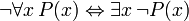
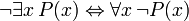
The following sentences can be called "identities" because the main connective in each is the biconditional. They are all provable in FOL, and are useful when manipulating the quantifiers:


 (where
  must not occur free in
  )
) (where must not occur free in )
Provable inference rules
The main connective in the following sentences, also provable in FOL, is the conditional. These sentences can be seen as the justification for inference rules in addition to modus ponens and universal generalization discussed above and assumed valid:


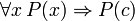 (If c is a variable, then it must not be previously quantified in P(x))
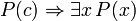 (there must be no free instance of x in P(c))
Metalogical theorems of first-order logic
Some important metalogical theorems are listed below in bulleted form. What they roughly mean is that a sentence is valid if and only if it is provable. Furthermore, one can construct an algorithm which works as follows: if a sentence is provable, the algorithm will tell us that in a finite but unknown amount of time. If a sentence is unprovable, the algorithm will run forever, and we will not know whether the sentence is unprovable or provable and the algorithm has just not yet told us that. Such an algorithm is called semidecidable or recursively enumerable.
One may construct an algorithm which will determine in finite number of steps whether a sentence is provable (a decidable algorithm) only for simple classes of first-order logic.
- The decision problem for validity is recursively enumerable; in other words, there is a Turing machine that when given any sentence as input, will halt if and only if the sentence is valid (true in all models).
- As Gödel's completeness theorem shows, for any valid formula P, P is provable. Conversely, assuming consistency of the logic, any provable formula is valid.
- The Turing machine can be one which generates all provable formulas in the following manner: for a finite or recursively enumerable set of axioms, such a machine can be one that generates an axiom, then generates a new provable formula by application of axioms and inference rules already generated, then generate another axiom, and so on. Given a sentence as input, the Turing machine simply go on and generates all provable formulas one by one, and will halt if it generates the sentence.
- Unlike the propositional logic, first-order logic is undecidable, provided that the language has at least one predicate of valence at least 2 other than equality. This means that there is no decision procedure that correctly determines whether an arbitrary formula is valid. Because there is a Turing machine as described above, the undecidability is related to the unsolvability of the Halting problem: there is no algorithm which determines after a finite number of steps whether the Turing machine will ever halt for a given sentence as its input, hence whether the sentence is provable. This result was established independently by Church and Turing.
- Monadic predicate logic (i.e., predicate logic with only predicates of one argument and no functions) is decidable.
- The Bernays–Schönfinkel class of first-order formulas is also decidable.
Translating natural language to first-order logic
Concepts expressed in natural language must be "translated" to first-order logic (FOL) before FOL can be used to address them, and there are a number of potential pitfalls in this translation. In FOL,  means "p, or q, or both", that is, it is inclusive. In English, the word "or" is sometimes inclusive (e.g, "cream or sugar?"), but sometimes it is exclusive (e.g., "coffee or tea?" is usually intended to mean one or the other, not both). Similarly, the English word "some" may mean "at least one, possibly all", but other times it may mean "not all, possibly none". The English word "and" should sometimes be translated as "or" (e.g., "men and women may apply").
Limitations of first-order logic
All mathematical notations have their strengths and weaknesses; here are a few such issues with first-order logic.
Difficulty representing if-then-else
Oddly enough, FOL with equality (as typically defined) does not include or permit defining an if-then-else predicate or function if(c,a,b), where "c" is a condition expressed as a formula, while a and b are either both terms or both formulas, and its result would be "a" if c is true, and "b" if it is false. The problem is that in FOL, both predicates and functions can only accept terms ("non-booleans") as parameters, but the "obvious" representation of the condition is a formula ("boolean"). This is unfortunate, since many mathematical functions are conveniently expressed in terms of if-then-else, and if-then-else is fundamental for describing most computer programs.
Mathematically, it is possible to redefine a complete set of new functions that match the formula operators, but this is quite clumsy. A predicate if(c,a,b) can be expressed in FOL if rewritten as  , but this is clumsy if the condition c is complex. Many extend FOL to add a special-case predicate named "if(condition, a, b)" (where a and b are formulas) and/or function "ite(condition, a, b)" (where a and b are terms), both of which accept a formula as the condition, and are equal to "a" if condition is true and "b" if it is false. These extensions make FOL easier to use for some problems, and make some kinds of automatic theorem-proving easier. Others extend FOL further so that functions and predicates can accept both terms and formulas at any position.
Typing (Sorts)
FOL does not include types (sorts) into the notation itself, other than the difference between formulas ("booleans") and terms ("non-booleans"). Some argue that this lack of types is a great advantage , but many others find advantages in defining and using types (sorts), such as helping reject some erroneous or undesirable specifications. Those who wish to indicate types must provide such information using the notation available in FOL. Doing so can make such expressions more complex, and can also be easy to get wrong.
Single-parameter predicates can be used to implement the notion of types where appropriate. For example, in: 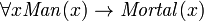 , the predicate
  could be considered a kind of "type assertion" (that is, that must be a man). Predicates can also be used with the "exists" quantifier to identify types, but this should usually be done with the "and" operator instead, e.g.:
 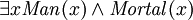 ("there exists something that is both a man and is mortal"). It is easy to write
  , but this would be equivalent to
  ("there is something that is not a man, and/or there exists something that is mortal"), which is usually not what was intended. Similarly, assertions can be made that one type is a subtype of another type, e.g.:
  ("for all , if is a man, then is a mammal").
Difficulty in characterizing finiteness or countability
It follows from the Löwenheim–Skolem theorem that it is not possible to characterize finiteness or countability in first-order logic. For example, in first-order logic one cannot assert the least-upper-bound property for sets of real numbers, which states that every bounded, nonempty set of real numbers has a supremum; A second-order logic is needed for that.
Graph reachability cannot be expressed
Many situations can be modeled as a graph of nodes and directed connections (edges). For example, validating many systems requires showing that a "bad" state cannot be reached from a "good" state, and these interconnections of states can often be modelled as a graph. However, it can be proved that connectedness cannot be fully expressed in predicate logic. In other words, there is no predicate-logic formula  and
and  as its only predicate symbol (of arity 2) such that holds in a interpretation
  if and only if the extension of in describes a connected graph: that is, connected graphs cannot be axiomatized.
Note that given a binary relation encoding a graph, one can describe in terms of a conjunction of first order formulas, and write a formula  which is satisfiable if and only if is connected.
Comparison with other logics
- Typed first-order logic allows variables and terms to have various types (or sorts). If there are only a finite number of types, this does not really differ much from first-order logic, because one can describe the types with a finite number of unary predicates and a few axioms. Sometimes there is a special type Ω of truth values, in which case formulas are just terms of type Ω.
- First-order logic with domain conditions adds domain conditions (DCs) to classical first-order logic, enabling the handling of partial functions; these conditions can be proven "on the side" in a manner similar to PVS's type correctness conditions. It also adds if-then-else to keep definitions and proofs manageable (they became too complex without them).
- The SMT-LIB Standard defines a language used by many research groups for satisfiability modulo theories; the full logic is based on FOL with equality, but adds sorts (types), if-then-else for terms and formulas (ite() and if.. then.. else..), a let construct for terms and formulas (let and flet), and a distinct construct declaring a set of listed values as distinct. Its connectives are not, implies, and, or, xor, and iff.
- Weak second-order logic allows quantification over finite subsets.
- Monadic second-order logic allows quantification over subsets, or in other words over unary predicates.
- Second-order logic allows quantification over subsets and relations, or in other words over all predicates. For example, the axiom of extensionality can be stated in second-order logic as x = y ≡def P (P(x) ↔ P(y)). The strong semantics of second-order logic give such sentences a much stronger meaning than first-order semantics.
- Higher-order logics allows quantification over higher types than second-order logic permits. These higher types include relations between relations, functions from relations to relations between relations, etc.
- Intuitionistic first-order logic uses intuitionistic rather than classical propositional calculus; for example, ¬¬φ need not be equivalent to φ. Similarly, first-order fuzzy logics are first-order extensions of propositional fuzzy logics rather than classical logic.
- Modal logic has extra modal operators with meanings which can be characterised informally as, for example "it is necessary that φ" and "it is possible that φ".
- In monadic predicate calculus predicates are restricted to having only one argument.
- Infinitary logic allows infinitely long sentences. For example, one may allow a conjunction or disjunction of infinitely many formulas, or quantification over infinitely many variables. Infinitely long sentences arise in areas of mathematics including topology and model theory.
- First-order logic with extra quantifiers has new quantifiers Qx,..., with meanings such as "there are many x such that ...". Also see branching quantifiers and the plural quantifiers of George Boolos and others.
- Predicate Logic with Definitions (PLD, or D-logic) modifies FOL by formally adding syntactic definitions as a type of value (in addition to formulas and terms); these definitions can be used inside terms and formulas.
- Independence-friendly logic is characterized by branching quantifiers, which allow one to express independence between quantified variables.
Most of these logics are in some sense extensions of FOL: they include all the quantifiers and logical operators of FOL with the same meanings. Lindström showed that FOL has no extensions (other than itself) that satisfy both the compactness theorem and the downward Löwenheim–Skolem theorem. A precise statement of Lindström's theorem requires a few technical conditions that the logic is assumed to satisfy; for example, changing the symbols of a language should make no essential difference to which sentences are true.
Algebraizations
Three ways of eliminating quantified variables from FOL, and that do not involve replacing quantifiers with other variable binding term operators, are known:
- Cylindric algebra, by Alfred Tarski and his coworkers;
- Polyadic algebra, by Paul Halmos;
- Predicate functor logic, mainly due to Willard Quine.
These algebras:
- Are all proper extensions of the two-element Boolean algebra, and thus are lattices;
- Do for FOL what Lindenbaum-Tarski algebra does for sentential logic;
- Allow results from abstract algebra, universal algebra, and order theory to be brought to bear on FOL.
Tarski and Givant (1987) show that the fragment of FOL that has no atomic sentence lying in the scope of more than three quantifiers, has the same expressive power as relation algebra. This fragment is of great interest because it suffices for Peano arithmetic and most axiomatic set theory, including the canonical ZFC. They also prove that FOL with a primitive ordered pair is equivalent to a relation algebra with two ordered pair projection functions.
Automation
Theorem proving for first-order logic is one of the most mature subfields of automated theorem proving. The logic is expressive enough to allow the specification of arbitrary problems, often in a reasonably natural and intuitive way. On the other hand, it is still semidecidable, and a number of sound and complete calculi have been developed, enabling fully automated systems. In 1965 J. Alan Robinson achieved an important breakthrough with his resolution approach; to prove a theorem it tries to refute the negated theorem, in a goal-directed way, resulting in a much more efficient method to automatically prove theorems in FOL. More expressive logics, such as higher-order and modal logics, allow the convenient expression of a wider range of problems than first-order logic, but theorem proving for these logics is less well developed.
A modern and particularly disruptive new technology is that of SMT solvers, which add arithmetic and propositional support to the powerful classes of SAT solvers.