Renormalization

Related subjects: Physics

About this schools Wikipedia selection

This wikipedia selection has been chosen by volunteers helping SOS Children from Wikipedia for this Wikipedia Selection for schools. Click here for more information on SOS Children.

Quantum field theory
Feynman diagram
History
Background Field theory Gauge theory Poincaré symmetry Quantum mechanics Spontaneous symmetry breaking
Symmetries Charge conjugation Crossing Parity Time reversal
Tools Anomaly Effective field theory Expectation value Faddeev–Popov ghosts Feynman diagram Lattice gauge theory LSZ reduction formula Partition function Propagator Quantization Regularization Renormalization Vacuum state Wick's theorem Wightman axioms
Equations Dirac equation Klein–Gordon equation Proca equations Wheeler–DeWitt equation Bargmann–Wigner equations
Standard Model Electroweak interaction Higgs mechanism Quantum chromodynamics Quantum electrodynamics Yang–Mills theory
Incomplete theories Quantum gravity String theory Supersymmetry Technicolor Theory of everything
Scientists C. D. Anderson P. W. Anderson Bardeen Bethe Bjorken Bogoliubov Brout Cabibbo Callan Cronin DeWitt Dirac Dyson Englert Fermi Feynman Fierz Fisher Fock Fröhlich Gell-Mann Gross Hänsch Heisenberg Higgs Haag 't Hooft Kadanoff Kendall Klitzing Kobayashi Lamb Landau Lee Majorana Maskawa Mills Nambu Nishijima Parisi Paul Polyakov Salam Schwinger Shockley Skyrme Störmer Sudarshan Thomson Tomonaga Veltman Ward Weinberg Wilczek Wilson Yang Yukawa

In quantum field theory, the statistical mechanics of fields, and the theory of self-similar geometric structures, renormalization refers to a collection of techniques used to take a continuum limit.

When describing space and time as a continuum, certain statistical and quantum mechanical constructions are ill defined. In order to define them, the continuum limit has to be taken carefully.

Renormalization determines the relationship between parameters in the theory, when the parameters describing large distance scales differ from the parameters describing small distances. Renormalization was first developed in quantum electrodynamics (QED) to make sense of infinite integrals in perturbation theory. Initially viewed as a suspect, provisional procedure by some of its originators, renormalization eventually was embraced as an important and self-consistent tool in several fields of physics and mathematics.

Self-interactions in classical physics

Figure 1. Renormalization in quantum electrodynamics: The simple electron-photon interaction that determines the electron's charge at one renormalization point is revealed to consist of more complicated interactions at another.

The problem of infinities first arose in the classical electrodynamics of point particles in the 19th and early 20th century.

The mass of a charged particle should include the mass-energy in its electrostatic field. Assume that the particle is a charged spherical shell of radius $r_e$ . The energy in the field is

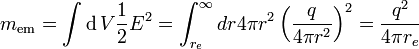
$m_\mathrm{em} = \int \operatorname{d}V {1\over 2}E^2 = \int_{r_e}^\infty dr 4\pi r^2 \left( {q\over 4\pi r^2} \right) ^2 = {q^2 \over 4\pi r_e}$

and it is infinite when $r_e$ is zero. The value of $r_e$ that makes $m_{\mathrm{em}}$ equal to the electron mass is called the classical electron radius. With factors of c and $\epsilon_0$ restored:

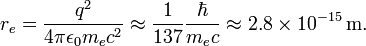
$r_e = {q^2 \over 4\pi\epsilon_0 m_e c^2} \approx {1\over 137}{\hbar\over m_e c} \approx 2.8 \times 10^{-15} \, \mathrm{m}.$

It is thus $\alpha$ times smaller than the Compton wavelength of the electron.

The mass of a spherical charged particle includes the mass of the spherical shell. If the shell's mass is allowed to be negative, it might be possible to take a consistent point limit. This was called renormalization, and Lorentz and Abraham attempted to develop a classical theory of the electron this way. This early work was the inspiration for later attempts at regularization and renormalization in quantum field theory.

When calculating the electromagnetic interactions of charged particles, it is tempting to ignore the back-reaction of a particle's own field on itself. But this back reaction is necessary to explain the friction on charged particles when they emit radiation. If the electron is assumed to be a point, the value of the back-reaction diverges, for the same reason that the mass diverges, because the field is inverse-square.

The Abraham-Lorentz theory had a noncausal "pre-acceleration". Sometimes an electron would start moving before the force is applied. This is a sign that the point limit is inconsistent. An extended body will start moving when a force is applied within one radius of the centre of mass.

The trouble was worse in classical field theory than in quantum field theory, because in quantum field theory a charged particle at short distances can fluctuate into an antiparticle. The antiparticle has opposite charge, and the fluctuations smear out the charge over a region comparable to the Compton wavelength. In quantum electrodynamics at small coupling the electromagnetic mass only diverges as the log of the radius of the particle.

Many physicists believe that when the fine structure constant is much greater than one, so that the classical electron radius is bigger than the quantum wavelength, the same problems that plague classical electrodynamics are still present in quantum electrodynamics.

Divergences in quantum electrodynamics

Figure 2. A diagram contributing to electron-electron scattering in QED. The loop has an ultraviolet divergence.

Vacuum polarization, a.k.a. charge screening. This loop has a logarithmic ultraviolet divergence.

Self energy diagram in QED.

When developing quantum electrodynamics in the 1930s, Max Born, Werner Heisenberg, Pascual Jordan, and Paul Dirac discovered that in perturbative calculations many integrals were divergent.

One way of describing the divergences was discovered in the 1930s by Ernst Stueckelberg, in the 1940s by Julian Schwinger, Richard Feynman, and Shin'ichiro Tomonaga, and systematized by Freeman Dyson. The divergences appear in calculations involving Feynman diagrams with closed loops of virtual particles in them.

While virtual particles obey conservation of energy and momentum, they can have any energy and momentum, even one that is not allowed by the relativistic energy-momentum relation for the observed mass of that particle. (That is, $E^2-p^2$ is not necessarily the mass of the particle in that process (e.g. for a photon it could be nonzero).) Such a particle is called off-shell. When there is a loop, the momentum of the particles involved in the loop is not uniquely determined by the energies and momenta of incoming and outgoing particles. A variation in the energy of one particle in the loop can be balanced by an equal and opposite variation in the energy of another particle in the loop. So to find the amplitude for the loop process one must integrate over all possible combinations of energy and momentum that could travel around the loop.

These integrals are often divergent, that is, they give infinite answers. The divergences which are significant are the " ultraviolet" (UV) ones. An ultraviolet divergence can be described as one which comes from

- the region in the integral where all particles in the loop have large energies and momentum.

- very short wavelengths and high frequencies fluctuations of the fields, in the path integral for the field.

- Very short proper-time between particle emission and absorption, if the loop is thought of as a sum over particle paths.

So these divergences are short-distance, short-time phenomena.

There are exactly three one-loop divergent loop diagrams in quantum electrodynamics.

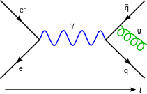
a photon creates a virtual electron- positron pair which then annihilate, this is a vacuum polarization diagram.
an electron which quickly emits and reabsorbs a virtual photon, called a self-energy.
An electron emits a photon, emits a second photon, and reabsorbs the first. This process is shown in figure 2, and it is called a vertex renormalization.

The three divergences correspond to the three parameters in the theory:

the field normalization Z.
the mass of the electron.
the charge of the electron.

A second class of divergence, called an infrared divergence, is due to massless particles, like the photon. Every process involving charged particles emits infinitely many coherent photons of infinite wavelength, and the amplitude for emitting any finite number of photons is zero. For photons, these divergences are well understood and are not a source of controversy.

A loop divergence

The diagram in Figure 2 shows one of the several one-loop contributions to electron-electron scattering in QED. The electron on the left side of the diagram, represented by the solid line, starts out with four-momentum $p^\mu$ and ends up with four-momentum $r^\mu$ . It emits a virtual photon carrying $r^\mu - p^\mu$ to transfer energy and momentum to the other electron. But in this diagram, before that happens, it emits another virtual photon carrying four-momentum $q^\mu$ , and it reabsorbs this one after emitting the other virtual photon. Energy and momentum conservation do not determine the four-momentum $q^\mu$ uniquely, so all possibilities contribute equally and we must integrate.

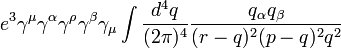
This diagram's amplitude ends up with, among other things, a factor from the loop of

$-ie^3 \int {d^4 q \over (2\pi)^4} \gamma^\mu {i (\gamma^\alpha (r-q)_\alpha + m) \over (r-q)^2 - m^2 + i \epsilon} \gamma^\rho {i (\gamma^\beta (p-q)_\beta + m) \over (p-q)^2 - m^2 + i \epsilon} \gamma^\nu {-i g_{\mu\nu} \over q^2 + i\epsilon }$

The various $\gamma^\mu$ factors in this expression are gamma matrices as in the covariant formulation of the Dirac equation; they have to do with the spin of the electron. The factors of $e$ are the electric coupling constant, while the $i\epsilon$ provide a heuristic definition of the contour of integration around the poles in the space of momenta. The important part for our purposes is the dependency on $q^\mu$ of the three big factors in the integrand, which are from the propagators of the two electron lines and the photon line in the loop.

This has a piece with two powers of $q^\mu$ on top that dominates at large values of $q^\mu$ (Pokorski 1987, p. 122):

$e^3 \gamma^\mu \gamma^\alpha \gamma^\rho \gamma^\beta \gamma_\mu \int {d^4 q \over (2\pi)^4}{q_\alpha q_\beta \over (r-q)^2 (p-q)^2 q^2}$

This integral is divergent, and infinite unless we cut it off at finite energy and momentum in some way.

Similar loop divergences occur in other quantum field theories.

Renormalized and bare quantities

The solution was to realize that the quantities initially appearing in the theory's formulae (such as the formula for the Lagrangian), representing such things as the electron's electric charge and mass, as well as the normalizations of the quantum fields themselves, did not actually correspond to the physical constants measured in the laboratory. As written, they were bare quantities that did not take into account the contribution of virtual-particle loop effects to the physical constants themselves. Among other things, these effects would include the quantum counterpart of the electromagnetic back-reaction that so vexed classical theorists of electromagnetism. In general, these effects would be just as divergent as the amplitudes under study in the first place; so finite measured quantities would in general imply divergent bare quantities.

In order to make contact with reality, then, the formulae would have to be rewritten in terms of measurable, renormalized quantities. The charge of the electron, say, would be defined in terms of a quantity measured at a specific kinematic renormalization point or subtraction point (which will generally have a characteristic energy, called the renormalization scale or simply the energy scale). The parts of the Lagrangian left over, involving the remaining portions of the bare quantities, could then be reinterpreted as counterterms, involved in divergent diagrams exactly canceling out the troublesome divergences for other diagrams.

Renormalization in QED

Figure 3. The vertex corresponding to the Z₁ counterterm cancels the divergence in Figure 2.

For example, in the Lagrangian of QED

$\mathcal{L}=\bar\psi_B\left[i\gamma_\mu (\partial^\mu + ie_BA_B^\mu)-m_B\right]\psi_B -\frac{1}{4}F_{B\mu\nu}F_B^{\mu\nu}$

the fields and coupling constant are really bare quantities, hence the subscript $B$ above. Conventionally the bare quantities are written so that the corresponding Lagrangian terms are multiples of the renormalized ones:

$\left(\bar\psi m \psi\right)_B = Z_0 \, \bar\psi m \psi$

$\left(\bar\psi (\partial^\mu + ieA^\mu)\psi\right)_B = Z_1 \, \bar\psi(\partial^\mu + ieA^\mu)\psi$

$\left(F_{\mu\nu}F^{\mu\nu}\right)_B = Z_3\, F_{\mu\nu}F^{\mu\nu}$ .

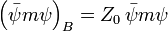
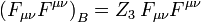( Gauge invariance, via a Ward-Takahashi identity, turns out to imply that we can renormalize the two terms of the covariant derivative piece 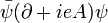$\bar \psi (\partial + ieA) \psi$ together (Pokorski 1987, p. 115), which is what happened to $Z_2$ ; it is the same as $Z_1$ .)

A term in this Lagrangian, for example, the electron-photon interaction pictured in Figure 1, can then be written

$\mathcal{L}_I = -e \bar\psi \gamma_\mu A^\mu \psi \, - \, (Z_1 - 1) e \bar\psi \gamma_\mu A^\mu \psi$

The physical constant $e$ , the electron's charge, can then be defined in terms of some specific experiment; we set the renormalization scale equal to the energy characteristic of this experiment, and the first term gives the interaction we see in the laboratory (up to small, finite corrections from loop diagrams, providing such exotica as the high-order corrections to the magnetic moment). The rest is the counterterm. If we are lucky, the divergent parts of loop diagrams can all be decomposed into pieces with three or fewer legs, with an algebraic form that can be canceled out by the second term (or by the similar counterterms that come from $Z_0$ and $Z_3$ ). In QED, we are lucky: the theory is renormalizable (see below for more on this).

The diagram with the $Z_1$ counterterm's interaction vertex placed as in Figure 3 cancels out the divergence from the loop in Figure 2.

The splitting of the "bare terms" into the original terms and counterterms came before the renormalization group insights due to Kenneth Wilson. According to the renormalization group insights, this splitting is unnatural and unphysical.

Running constants

To minimize the contribution of loop diagrams to a given calculation (and therefore make it easier to extract results), one chooses a renormalization point close to the energies and momenta actually exchanged in the interaction. However, the renormalization point is not itself a physical quantity: the physical predictions of the theory, calculated to all orders, should in principle be independent of the choice of renormalization point, as long as it is within the domain of application of the theory. Changes in renormalization scale will simply affect how much of a result comes from Feynman diagrams without loops, and how much comes from the leftover finite parts of loop diagrams. One can exploit this fact to calculate the effective variation of physical constants with changes in scale. This variation is encoded by beta-functions, and the general theory of this kind of scale-dependence is known as the renormalization group.

Colloquially, particle physicists often speak of certain physical constants as varying with the energy of an interaction, though in fact it is the renormalization scale that is the independent quantity. This running does, however, provide a convenient means of describing changes in the behaviour of a field theory under changes in the energies involved in an interaction. For example, since the coupling constant in quantum chromodynamics becomes small at large energy scales, the theory behaves more like a free theory as the energy exchanged in an interaction becomes large, a phenomenon known as asymptotic freedom. Choosing an increasing energy scale and using the renormalization group makes this clear from simple Feynman diagrams; were this not done, the prediction would be the same, but would arise from complicated high-order cancellations.

Regularization

Since the quantity $\infty - \infty$ is ill-defined, in order to make this notion of canceling divergences precise, the divergences first have to be tamed mathematically using the theory of limits, in a process known as regularization.

An essentially arbitrary modification to the loop integrands, or regulator, can make them drop off faster at high energies and momenta, in such a manner that the integrals converge. A regulator has a characteristic energy scale known as the cutoff; taking this cutoff to infinity (or, equivalently, the corresponding length/time scale to zero) recovers the original integrals.

With the regulator in place, and a finite value for the cutoff, divergent terms in the integrals then turn into finite but cutoff-dependent terms. After canceling out these terms with the contributions from cutoff-dependent counterterms, the cutoff is taken to infinity and finite physical results recovered. If physics on scales we can measure is independent of what happens at the very shortest distance and time scales, then it should be possible to get cutoff-independent results for calculations.

Many different types of regulator are used in quantum field theory calculations, each with its advantages and disadvantages. One of the most popular in modern use is dimensional regularization, invented by Gerardus 't Hooft and Martinus J. G. Veltman, which tames the integrals by carrying them into a space with a fictitious fractional number of dimensions. Another is Pauli-Villars regularization, which adds fictitious particles to the theory with very large masses, such that loop integrands involving the massive particles cancel out the existing loops at large momenta.

Yet another regularization scheme is the Lattice regularization, introduced by Kenneth Wilson, which pretends that our space-time is constructed by hyper-cubical lattice with fixed grid size. This size is a natural cutoff for the maximal momentum that a particle could possess when propagating on the lattice. And after doing calculation on several lattices with different grid size, the physical result is extrapolated to grid size 0, or our natural universe. This presupposes the existence of a scaling limit.

A rigorous mathematical approach to renormalization theory is the so-called causal perturbation theory, where ultraviolet divergences are avoided from the start in calculations by performing well-defined mathematical operations only within the framework of distribution theory. The disadvantage of the method is the fact that the approach is quite technical and requires a high level of mathematical knowledge.

Zeta function regularization

Julian Schwinger discovered a relationship between zeta function regularization and renormalization, using the asymptotic relation:

$I(n, \Lambda )= \int_{0}^{\Lambda }dp\,p^{n} \sim 1+2^n+3^n+...+ \Lambda^n = \zeta(-n)$

as the regulator $\Lambda \rightarrow \infty$ . Based on this, he considered using the values of $\zeta(-n)$ to get finite results. Although he reached inconsistent results, an improved formula by Hartle, J. Garcia,E. Elizalde includes

$I(n, \Lambda) = \frac{n}{2}I(n-1, \Lambda) + \zeta(-n) - \sum_{r=1}^{\infty}\frac{B_{2r}}{(2r)!} a_{n,r}(n-2r+1) I(n-2r, \Lambda)$ ,

where the B's are the Bernoulli numbers and

$a_{n,r}= \frac{\Gamma(n+1)}{\Gamma(n-2r+2)}$ .

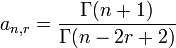So every $I(m,\Lambda )$ can be written as a linear combination of $\zeta(-1),\zeta(-3),\zeta(-5),...... \zeta(-m)$

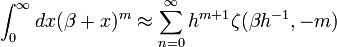
Or simply using Abel-Plana formula we have for every divergent integral:

$\zeta(-m, \beta )-\frac{\beta ^{m}}{2}-i\int_ 0 ^{\infty}dt \frac{ (it+\beta)^{m}-(-it+\beta)^{m}}{e^{2 \pi t}-1}=\int_0 ^{\infty} dp (p+\beta)^{m}$ valid when m>0, Here the Zeta function is Hurwitz zeta function and Beta is a positive real number.

The "Geometric" analogy is given by, (if we use rectangle method) to evaluate the integral so:

$\int_{0}^{\infty}dx(\beta +x)^{m}\approx \sum_{n=0}^{\infty}h^{m+1} \zeta( \beta h^{-1} , -m)$

Using Hurwitz zeta regularization plus rectangle method with step h (not to be confused with Planck's constant)

Attitudes and interpretation

The early formulators of QED and other quantum field theories were, as a rule, dissatisfied with this state of affairs. It seemed illegitimate to do something tantamount to subtracting infinities from infinities to get finite answers.

Dirac's criticism was the most persistent. As late as 1975, he was saying:

Most physicists are very satisfied with the situation. They say: 'Quantum electrodynamics is a good theory and we do not have to worry about it any more.' I must say that I am very dissatisfied with the situation, because this so-called 'good theory' does involve neglecting infinities which appear in its equations, neglecting them in an arbitrary way. This is just not sensible mathematics. Sensible mathematics involves neglecting a quantity when it is small - not neglecting it just because it is infinitely great and you do not want it!

Another important critic was Feynman. Despite his crucial role in the development of quantum electrodynamics, he wrote the following in 1985:

The shell game that we play ... is technically called 'renormalization'. But no matter how clever the word, it is still what I would call a dippy process! Having to resort to such hocus-pocus has prevented us from proving that the theory of quantum electrodynamics is mathematically self-consistent. It's surprising that the theory still hasn't been proved self-consistent one way or the other by now; I suspect that renormalization is not mathematically legitimate.

While Dirac's criticism was based on the procedure of renormalization itself, Feynman's criticism was very different. Feynman was concerned that all field theories known in the 1960s had the property that the interactions becomes infinitely strong at short enough distance scales. This property, called a Landau pole, made it plausible that quantum field theories were all inconsistent. In 1974, Gross, Politzer and Wilczek showed that another quantum field theory, Quantum Chromodynamics, does not have a landau pole. Feynman, along with most others, accepted that QCD was a fully consistent theory.

The general unease was almost universal in texts up to the 1970s and 1980s. Beginning in the 1970s, however, inspired by work on the renormalization group and effective field theory, and despite the fact that Dirac and various others -- all of whom belonged to the older generation -- never withdrew their criticisms, attitudes began to change, especially among younger theorists. Kenneth G. Wilson and others demonstrated that the renormalization group is useful in statistical field theory applied to condensed matter physics, where it provides important insights into the behaviour of phase transitions. In condensed matter physics, a real short-distance regulator exists: matter ceases to be continuous on the scale of atoms. Short-distance divergences in condensed matter physics do not present a philosophical problem, since the field theory is only an effective, smoothed-out representation of the behaviour of matter anyway; there are no infinities since the cutoff is actually always finite, and it makes perfect sense that the bare quantities are cutoff-dependent.

If QFT holds all the way down past the Planck length (where it might yield to string theory, causal set theory or something different), then there may be no real problem with short-distance divergences in particle physics either; all field theories could simply be effective field theories. In a sense, this approach echoes the older attitude that the divergences in QFT speak of human ignorance about the workings of nature, but also acknowledges that this ignorance can be quantified and that the resulting effective theories remain useful.

In QFT, the value of a physical constant, in general, depends on the scale that one chooses as the renormalization point, and it becomes very interesting to examine the renormalization group running of physical constants under changes in the energy scale. The coupling constants in the Standard Model of particle physics vary in different ways with increasing energy scale: the coupling of quantum chromodynamics and the weak isospin coupling of the electroweak force tend to decrease, and the weak hypercharge coupling of the electroweak force tends to increase. At the colossal energy scale of 10¹⁵ GeV (far beyond the reach of our civilization's particle accelerators), they all become approximately the same size (Grotz and Klapdor 1990, p. 254), a major motivation for speculations about grand unified theory. Instead of being only a worrisome problem, renormalization has become an important theoretical tool for studying the behaviour of field theories in different regimes.

If a theory featuring renormalization (e.g. QED) can only be sensibly interpreted as an effective field theory, i.e. as an approximation reflecting human ignorance about the workings of nature, then the problem remains of discovering a more accurate theory that does not have these renormalization problems. As Lewis Ryder has put it, "In the Quantum Theory, these [classical] divergences do not disappear; on the contrary, they appear to get worse. And despite the comparative success of renormalisation theory the feeling remains that there ought to be a more satisfactory way of doing things."

Renormalizability

From this philosophical reassessment a new concept follows naturally: the notion of renormalizability. Not all theories lend themselves to renormalization in the manner described above, with a finite supply of counterterms and all quantities becoming cutoff-independent at the end of the calculation. If the Lagrangian contains combinations of field operators of excessively high dimension in energy units, the counterterms required to cancel all divergences proliferate to infinite number, and, at first glance, the theory would seem to gain an infinite number of free parameters and therefore lose all predictive power, becoming scientifically worthless. Such theories are called nonrenormalizable.

The Standard Model of particle physics contains only renormalizable operators, but the interactions of general relativity become nonrenormalizable operators if one attempts to construct a field theory of quantum gravity in the most straightforward manner, suggesting that perturbation theory is useless in application to quantum gravity.

However, in an effective field theory, "renormalizability" is, strictly speaking, a misnomer. In a nonrenormalizable effective field theory, terms in the Lagrangian do multiply to infinity, but have coefficients suppressed by ever-more-extreme inverse powers of the energy cutoff. If the cutoff is a real, physical quantity—if, that is, the theory is only an effective description of physics up to some maximum energy or minimum distance scale—then these extra terms could represent real physical interactions. Assuming that the dimensionless constants in the theory do not get too large, one can group calculations by inverse powers of the cutoff, and extract approximate predictions to finite order in the cutoff that still have a finite number of free parameters. It can even be useful to renormalize these "nonrenormalizable" interactions.

Nonrenormalizable interactions in effective field theories rapidly become weaker as the energy scale becomes much smaller than the cutoff. The classic example is the Fermi theory of the weak nuclear force, a nonrenormalizable effective theory whose cutoff is comparable to the mass of the W particle. This fact may also provide a possible explanation for why almost all of the particle interactions we see are describable by renormalizable theories. It may be that any others that may exist at the GUT or Planck scale simply become too weak to detect in the realm we can observe, with one exception: gravity, whose exceedingly weak interaction is magnified by the presence of the enormous masses of stars and planets.

Renormalization schemes

In actual calculations, the counterterms introduced to cancel the divergences in Feynman diagram calculations beyond tree level must be fixed using a set of renormalization conditions. The common renormalization schemes in use include:

Minimal subtraction (MS) scheme and the related modified minimal subtraction (MS-bar) scheme
On-shell scheme

Application in Statistical Physics

As mentioned in the introduction, the methods of renormalization have been applied to Statistical Physics, namely to the problems of the critical behaviour near second-order phase transitions, in particular at fictitious spatial dimensions just below the number of 4, where the above-mentioned methods could even be sharpened (i.e., instead of "renormalizability" one gets "super-renormalizability"), which allowed extrapolation to the real spatial dimensionality for phase transitions, 3. Details can be found in the book of Zinn-Justin, mentioned below.

For the discovery of these unexpected applications, and working out the details, in 1982 the physics Noble prize was given to Kenneth G. Wilson.

Retrieved from " http://en.wikipedia.org/w/index.php?title=Renormalization&oldid=226641245"

We provide Linux to the World